ExaGOOP utilizes the formulation outlined in the previous section. This section presents validation and verification test cases using ExaGOOP.
Axial vibration of an elastic bar
In this test case, the free, axial vibration of a continuum bar made of a linearly elastic material is studied. This is one of the test cases for which the exact solution is known.
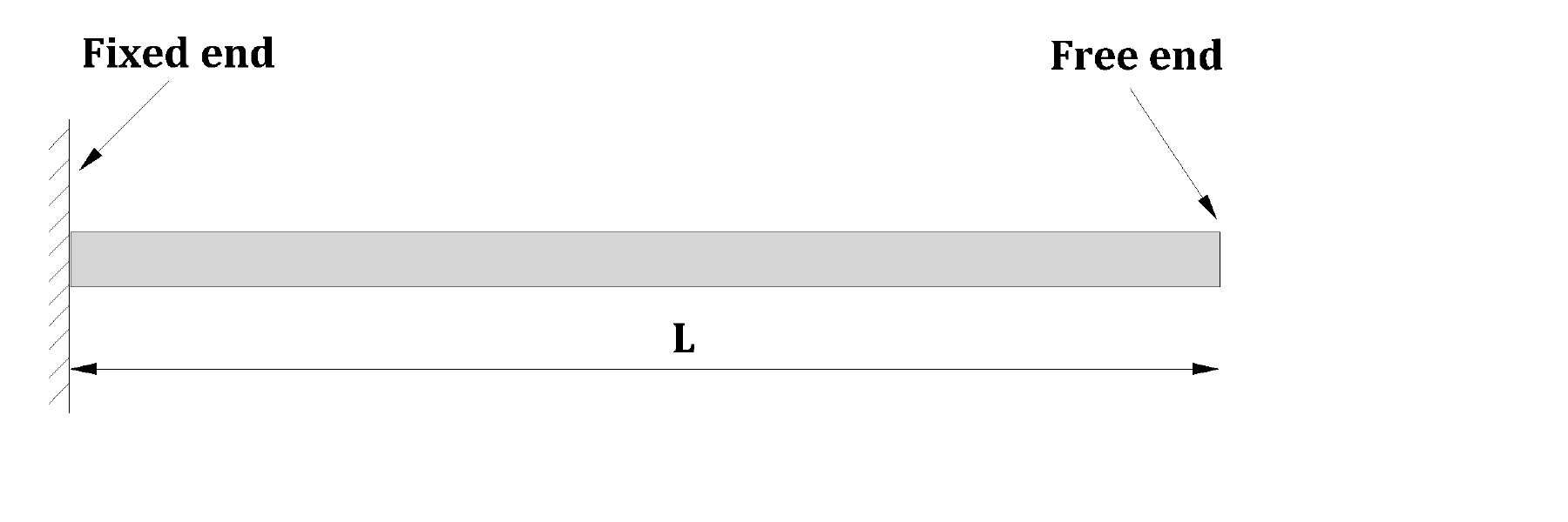
(a) The physical domain of the bar
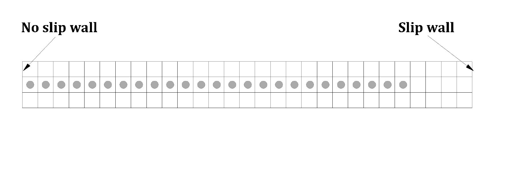
(b) Modeling of the bar in ExaGOOP

Fig. 3 Axial vibration of a bar. (a) Configuration of test case (b) Corresponding MPM model. Gray lines indicate the background Eulerian grid, and the gray circles are the material points located at time t = 0.
The test case configuration is shown in Fig. 3 (a). The bar has a length \(L\) with an area of cross-section \(A\) and is made up of a linear elastic material with Young’s modulus \(E\). The Poisson’s ratio of the material is set as zero. The bar is fixed at one end and left free at the other. The equation governing the vibration of the bar is given by,
where \(u\) is the axial displacement and \(c\) is the speed of sound in the elastic medium. The bar is subjected to the following boundary conditions:
When an initial axial velocity \(v(x,0)= V_0 \sin \left(\frac{\pi x}{2 L}\right)\) is imposed on the bar, the analytical solution to the governing equation Eq (6) subjected to the boundary conditions Eqs. (7) is given by,
where \(\omega_1\) is the fundamental frequency of the first mode of vibration.
Numerical simulations of this test case are performed using ExaGOOP. The properties of the bar are set as \(E=100, L=25\) and \(V_0 = 0.1\). The density of the material, \(\rho\) is set equal to unity. The length of the bar is discretized using \(25\) material points located equidistant from each other so that each material point simulates one unit length of the bar. Even though this test case involves only one-dimension in space, a three-dimensional, structured background grid with unit grid length is generated by ExaGOOP . The grid has \(29\) cells in the axial direction and three cells in the other two directions. At the initial time, each material point is located at the center of the cell as shown in Fig. 3 (b). Four grid cells are left as a buffer region between the right-most material point and the right boundary of the background grid. No-slip and slip wall boundary conditions are imposed on the left and the right boundaries, respectively, while periodic boundary conditions are imposed in the other two directions. Simulations are performed using both the linear-hat shape functions as well as the cubic B-spline shape functions, and for \(\alpha_{P-F}\) equal to zero and one, respectively. The CFL numbers are varied across different simulations. For ease of presentation, the comparisons between the exact solution and the MPM solutions obtained using are shown here using the center of mass velocity of the bar, \(v_{cm}\) and using system energies. The exact center of mass velocity is given by \(v_{\mathrm{cm}}^{\mathrm{exa}}(t)=\frac{V_0 c}{\omega_1 L} \cos \left(\omega_1 t\right)\) and its MPM counterpart is calculated as \(v_{\mathrm{cm}}^{\mathrm{num}}(t)=\frac{\sum v_p(t) m_p}{\sum m_p}\). Three different forms of system energy is shown for comparison, namely the kinetic energy (\(KE=\frac{1}{2} \sum_{p=1}^{n_p} \mathbf{v}_p \cdot \mathbf{v}_p m_p\)), the strain energy (\(SE=\frac{1}{2} \sum_{p=1}^{n_p} \sigma_{p} \epsilon_{p} V_p\)) and the total energy (\(TE=KE+SE\)).
Effect of \(\alpha_{P-F}\)
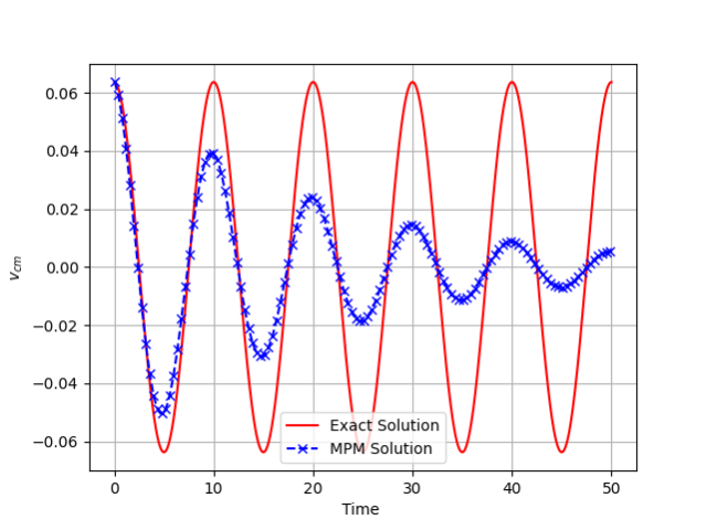
(a) alpha=0
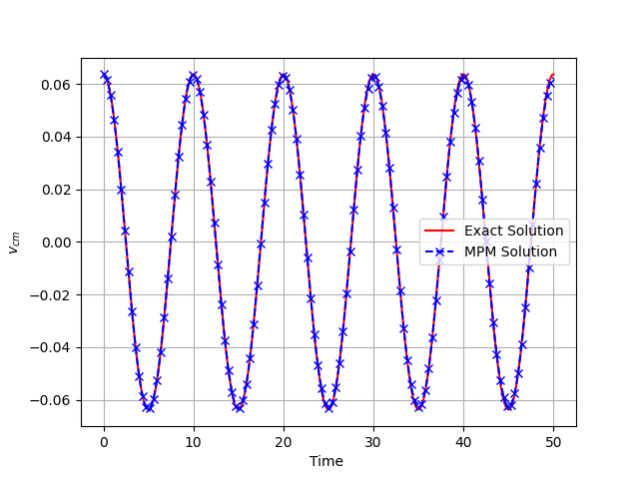
(b) alpha=1
Fig. 4 Effect of \(\alpha_{P-F}\) on the center of mass velocity of the axial bar
Fig. 4 shows the variation of \(v_{cm}\) as a function of time for two different values of \(\alpha_{P-F}\) (\(0\) and \(1\)). It is observed that for \(\alpha_{P-F}=0\), the center of mass velocity decreases with time in contrast to the exact solution where the amplitude remains unchanged. On the other hand, for \(\alpha_{P-F}=1\) the exact nature of the solution is well captured by ExaGOOP solution.
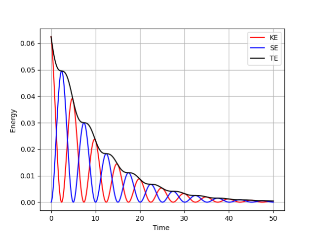
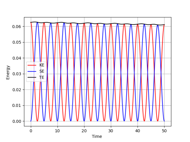
This dissipative nature of the numerical solution at low values of \(\alpha_{P-F}\) can also be observed from the temporal evolution of energies plotted in Fig. 5. Both kinetic and strain energy (and hence the total energy as well) is found to decrease and ultimately reach zero with time for \(\alpha_{P-F}=0\) while \(\alpha_{P-F}=1\) captures the non-dissipative nature of the exact solution accurately.
(a) alpha=0
(b) alpha=1
Fig. 5 Effect of \(\alpha_{P-F}\) on the kinetic (KE), strain (SE) and total (TE) of the axial bar
Effect of \(CFL\)
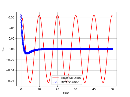
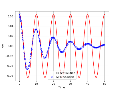
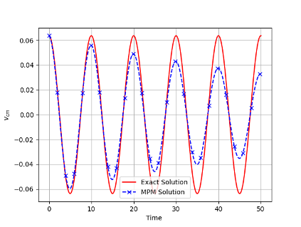
It is also interesting to study the effect of \(CFL\) on the solution accuracy. Fig. 6 shows the time evolution of \(v_{cm}\) for values of \(CFL=0.01,0.1\) and \(0.5\). The results shown are obtained using the cubic spline shape functions and for \(\alpha_{P-F}=0\). It is observed that the magnitude of \(v_{cm}\) reduces over time for this numerical parameters. It is also observed that the MPM solution deviates from the exact solution as the \(CFL\) is reduced. The solution is observed to be more dissipative as the CFL number is reduced. Results obtained using the linear hat shape functions also show a similar trend and hence are not shown here.
(a) CFL=0.01
(b) CFL=0.1
(b) CFL=0.5
Fig. 6 Effect of \(CFL\) on the center of mass velocity of the axial bar (alpha=0)
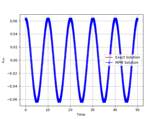
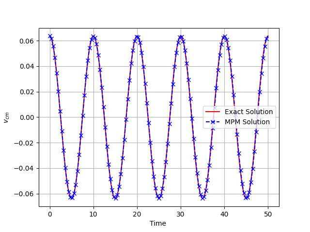
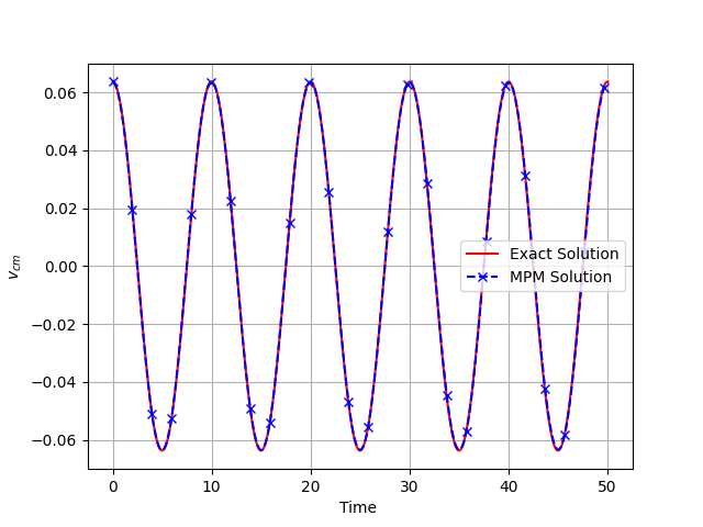
On the contrary, very minimal deviations from the exact solution are observed for all \(CFL\) numbers for \(\alpha_{P-F}=1\) as shown in Fig. 7. This again highlights the significance of chosing a high value of \(\alpha_{P-F}\) (0.9-1.0) for accurate simulations. This trend also holds for the solution computed using the linear hat shape functions.
(a) CFL=0.01
(b) CFL=0.1
(b) CFL=0.5
Fig. 7 Effect of \(CFL\) on the center of mass velocity of the axial bar (alpha=1)
Hence, it is concluded that lower values of \(\alpha_{P-F}\) lead to dissipative solution. The dissipative nature further worsens with smaller values of CFL number. Hence, for all MPM simulations a typical value of \(\alpha_{P-F}=0.95-1.0\) is suggested.
Collision of two-dimensional elastic disks
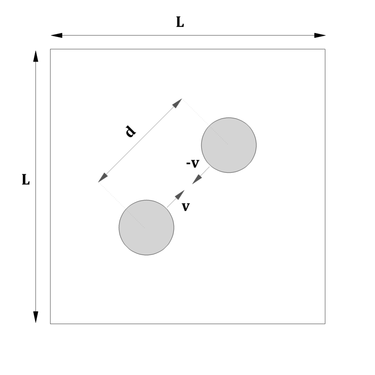
(a) Physical problem
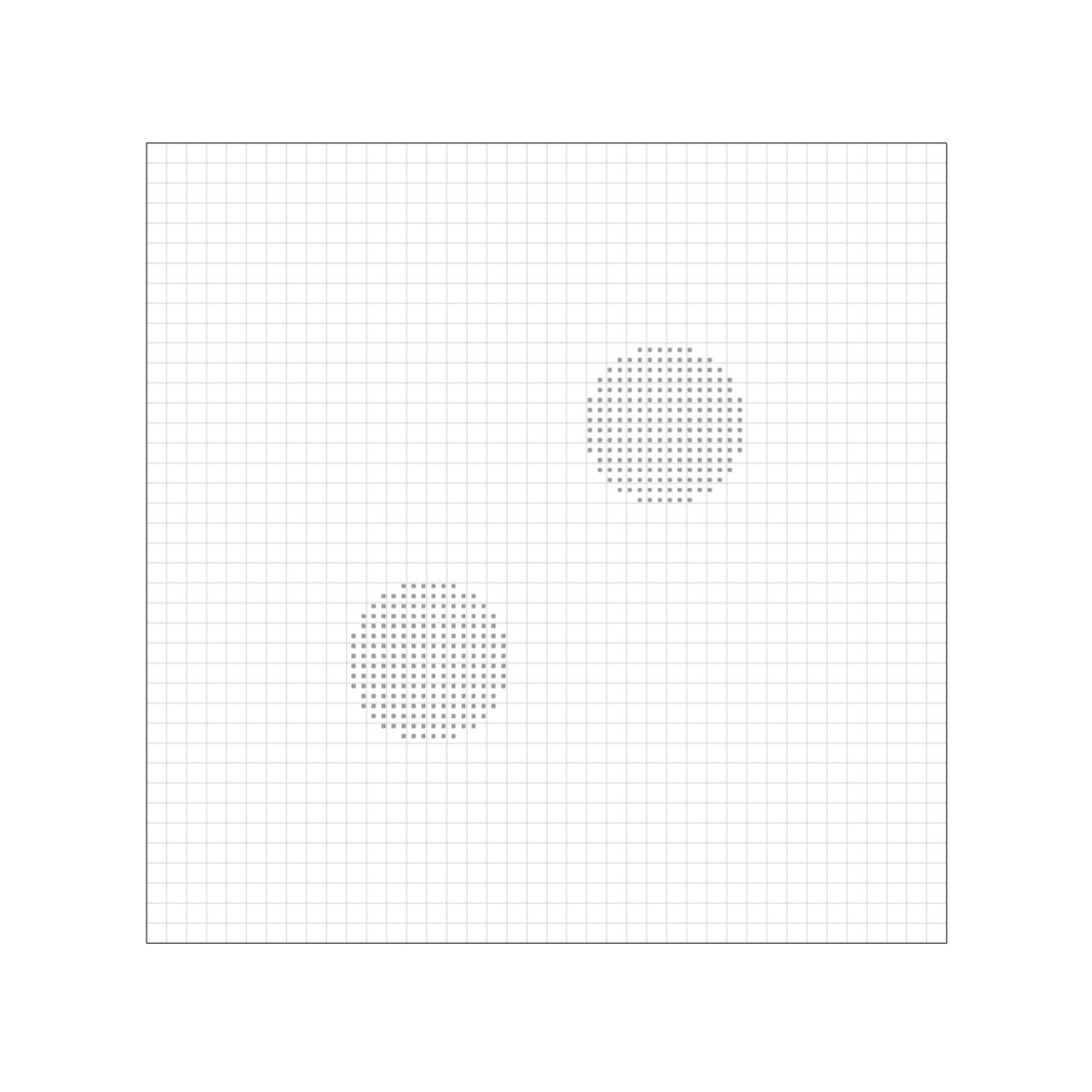
(b)ExaGOOP model
Fig. 8 Elastic collision of two circular disks. (a) Physical problem definition (b) ExaGOOP background grid and material points at time, t=0
This test case is used to verify ExaGOOP’s capability to simulate problems involving contact detection. The two-dimensional test case configuration is shown in Fig. 8 (a) and consists of two elastic disks, each of radius \(r\) and separated by a distance \(d\). At time \(t=0\), both the disks have a velocity \(v\) and are directed towards each other. As time progresses, both disks approach each other at constant velocity and collide. After collision, the disks rebound and move away from each other. Since the collision is elastic, the total energy of the disks remains constant in time.
For simulating this test case in ExaGOOP, the value of Young’s modulus \(E\) and density \(\rho\) is chosen as \(1000\). The Poisson’s ratio is set as 0.3. The radius of the disks is set to 0.2 m each and the disks are separated by a distance of \(d=0.6\sqrt{2}\) m. The background grid is a square of side \(L=2\)m and consists of 20 cells each in the x and y directions. The two disks are modeled using linear elastic material points with four material points located inside each cell. Simulations are carried out using both the linear hat and the cubic B-spline shape functions. Based on the conclusions from the previous test case, the value of CFL and \(\alpha_{P-F}\) are chosen as 0.1 and 0.95, respectively.
(a) t = 0
(b) t = 0.85
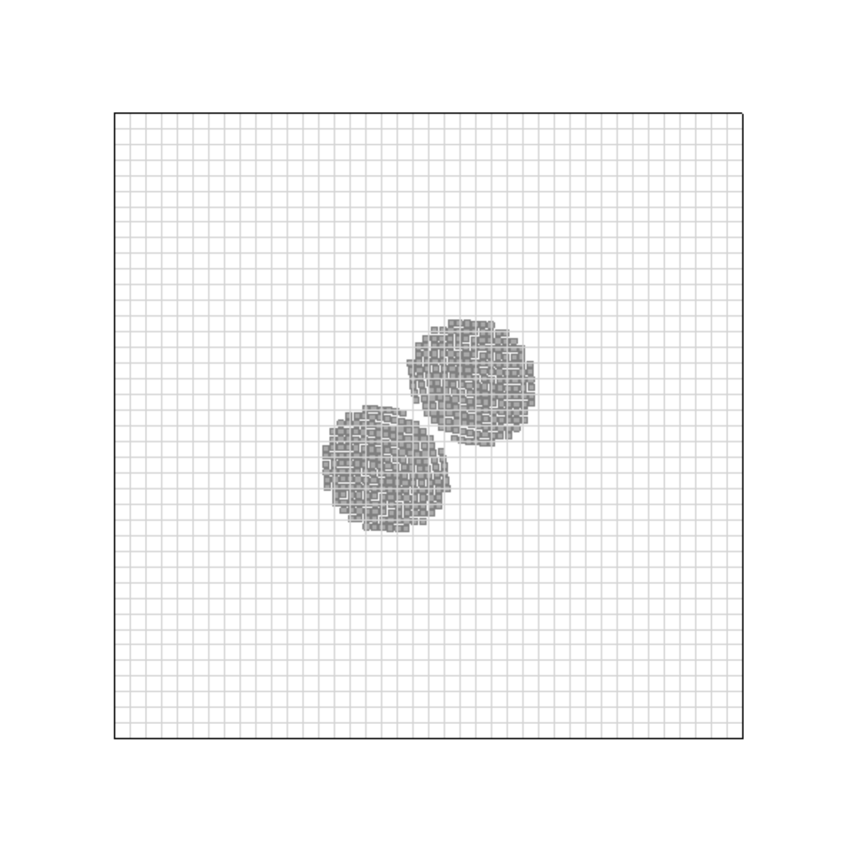
(c) t = 2.25
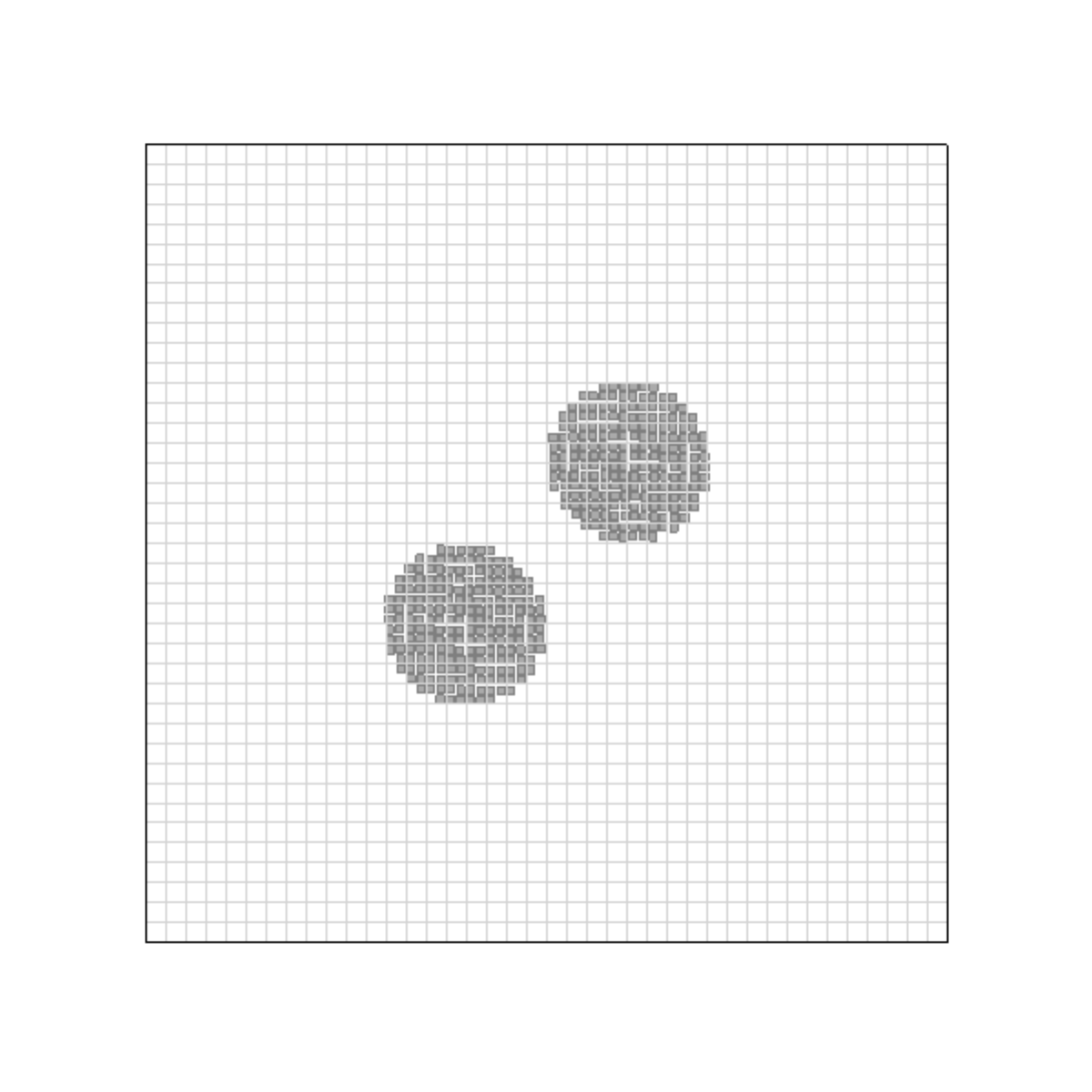
(d) t = 3.1
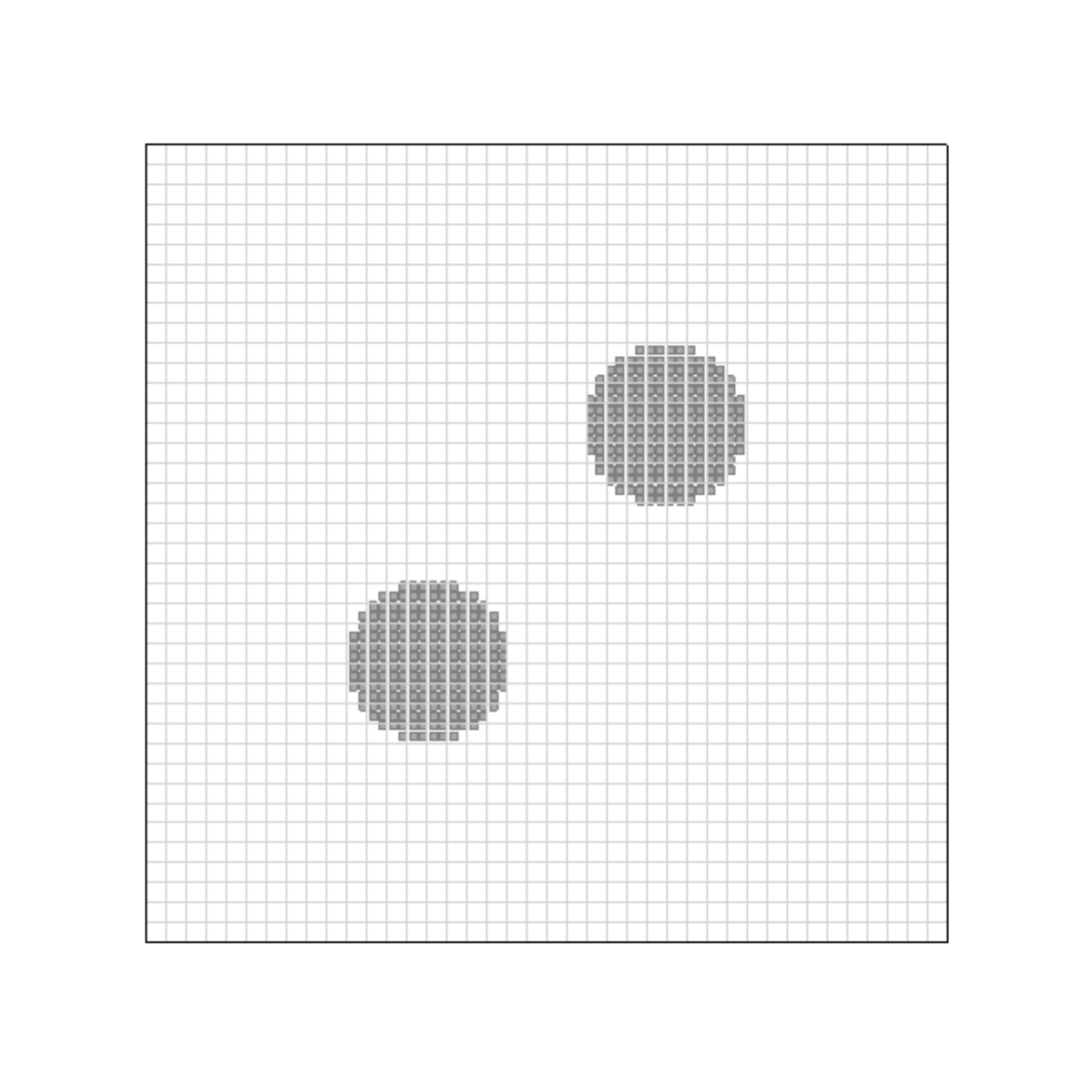
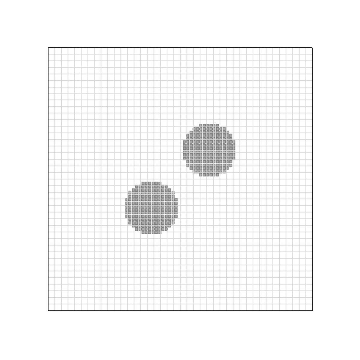
Fig. 9 Various stages of disks motion and collision simulated using ExaGOOP
Fig. 9 (a) and (b) show the approach of the disks towards each other. Fig. 9 (c) shows the instant at which the disks collide and Fig. 9 (d) shows the disks rebounding after collision.
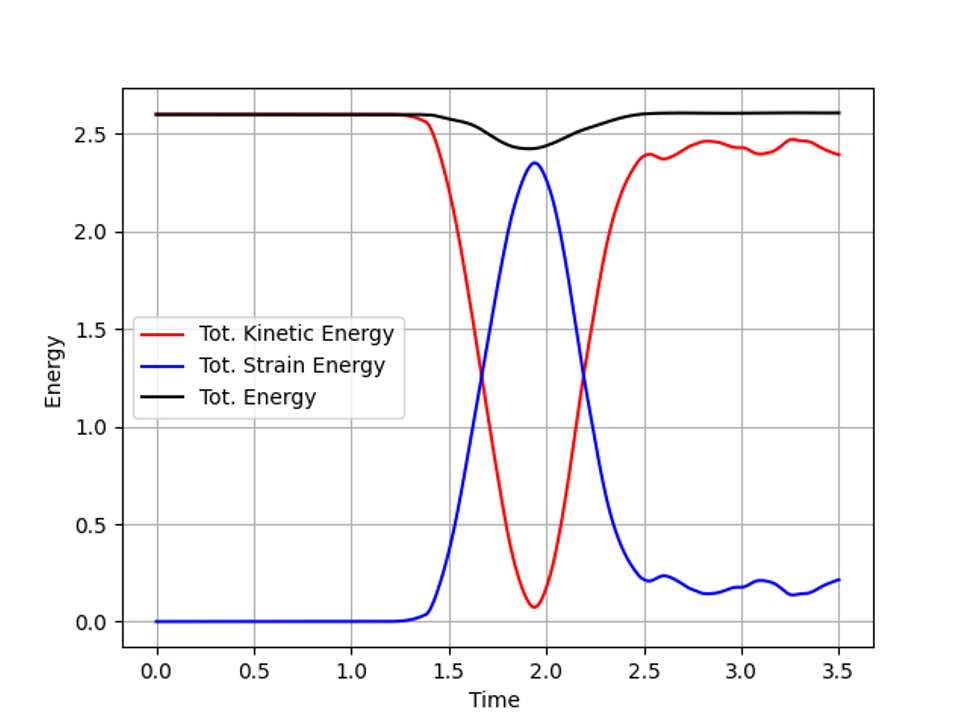
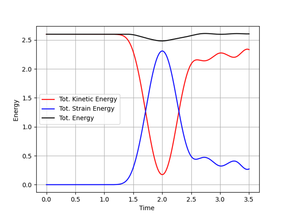
Fig. 10 (a) and (b) show the time evolution of the energies of both disks simulated using linear hat and cubic B-spline shape functions. From the initial time until the moment of collision, only kinetic energy exists for both disks due to their initial velocities.
(a) Linear hat shape function
(b) Cubic B-spline shape function
Fig. 10 Time evolution of kinetic, strain and total energies of both the disks
Once the disks collide, a portion of the total energy is converted to strain energy. Since there are no dissipative mechanisms modeled in this problem, the total energy of the disks should be conserved. Both the linear hat and the cubic spline shape function are able to recover the total energy completely. A temporary loss of total energy is observed during the time of collision. This is due to the mass lumping algorithm adopted which tend to make the solution slightly dissipative. The exact time of contact happens at time \(t=1.58\)sec while the numerical simulations tend to predict the contact much early. This is because, the contact in MPM occurs through the background grid nodes and not through material points. This inaccuracy can be reduced by refining the background grid further.
Dam break simulation
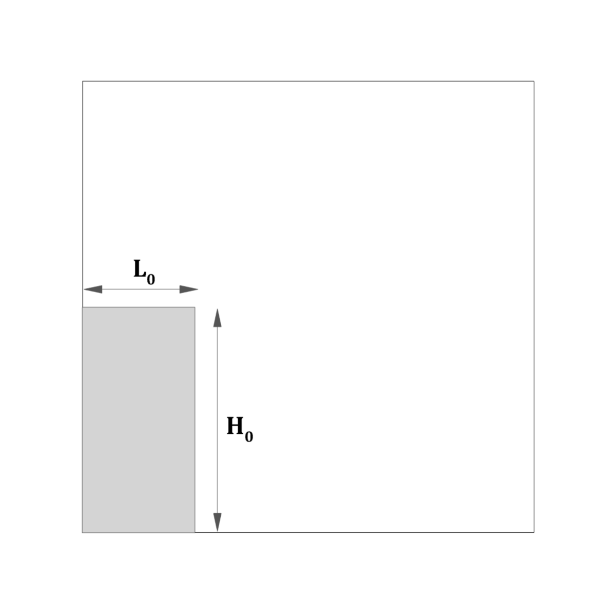
ExaGOOP’s capability in simulating fluids is demonstrated using the 2-D dam break test case. The test case consists of an initial column of water of height \(H_0\) and width \(L_0\) located inside a square domain, as shown in Fig. 11 (a). When \(t=0\), the water column is released, allowing it to flow downward due to gravity. Over time, the water gradually fills the entire domain. Experimental measurements of the water front are available [3] for comparison with MPM results.
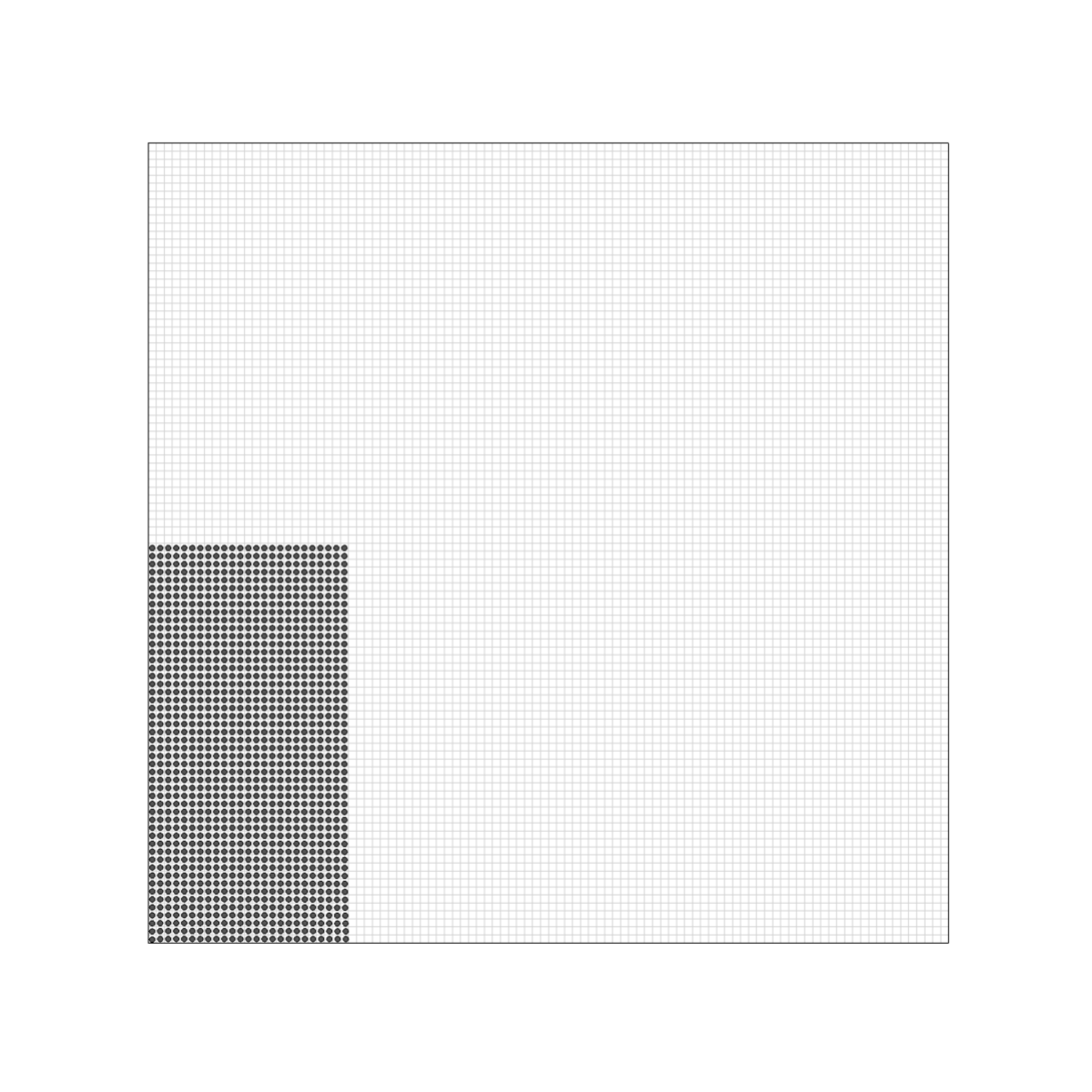
For the MPM simulations, the domain is structured as shown in Fig. 11 (b). A square domain with a side length of 0.4m is selected to create the background grid, which is discretized into 100 cells in each direction. The height of the water column is set at 0.2 m, and the width is 0.1 m. Unlike previous test cases discussed, water is treated as a fluid, necessitating the specification of an appropriate equation of state. In this study, water is modelled using a barotopic equation of state that relates pressure to the density of water as,
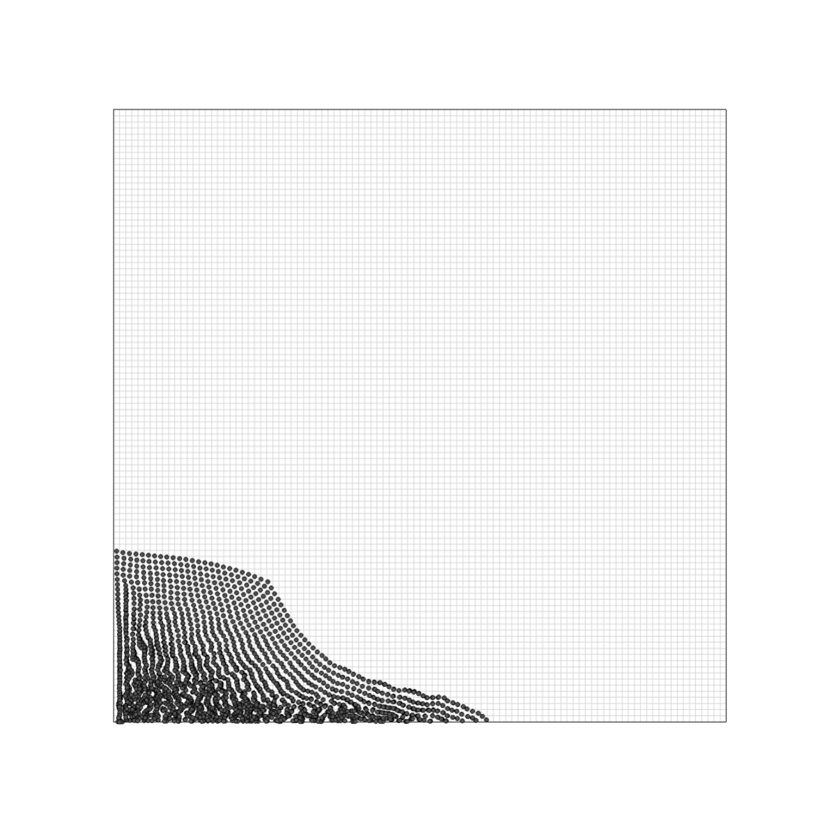
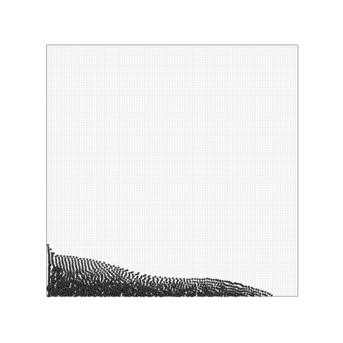
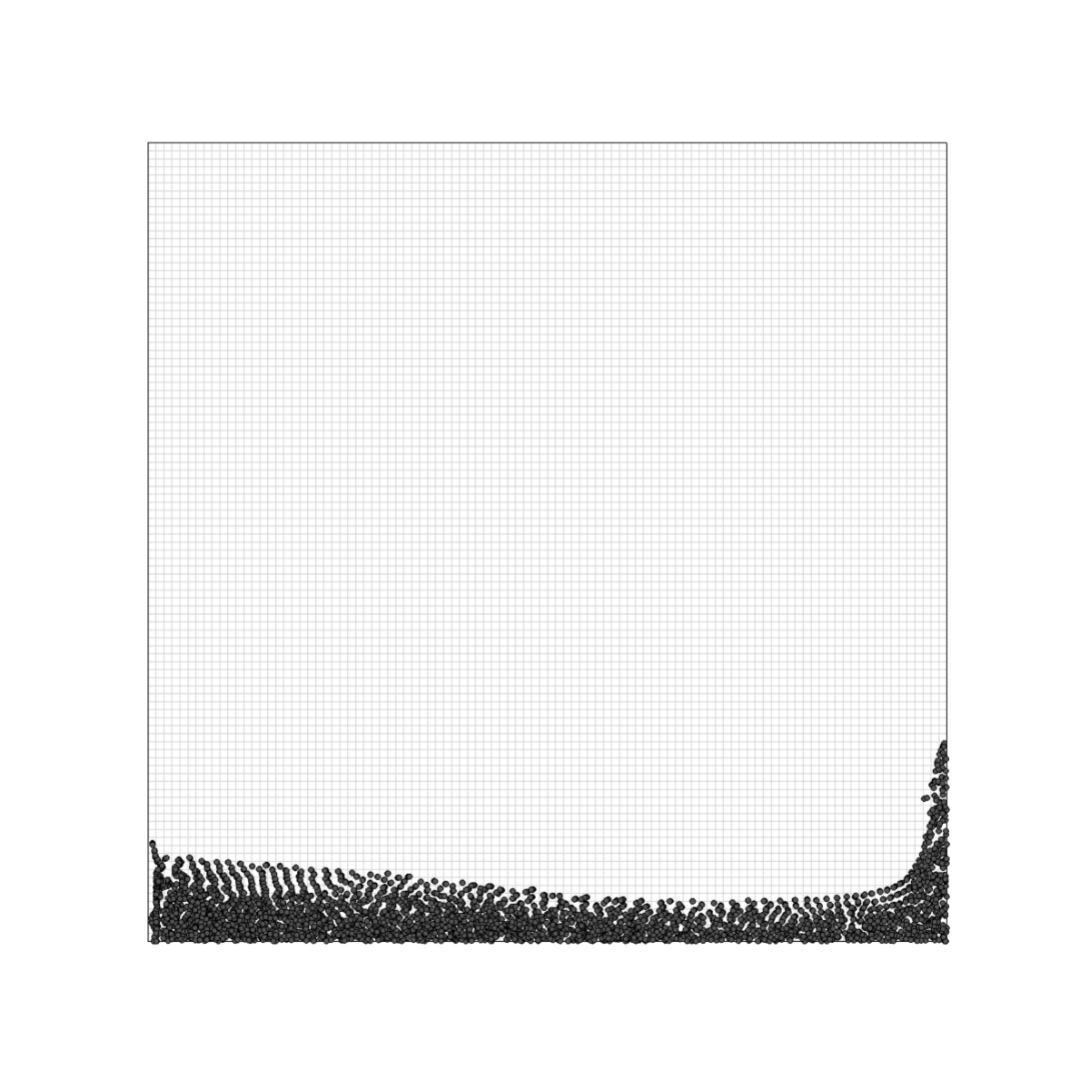
The value of \(\kappa\) and \(\gamma\) is set as 20000 and 7.0 respectively. The density of water is initialised as 1000 kg/m3. Simulation is performed using \(CFL=0.1\) and \(\alpha_{P-F}=0.95\). The spatial discretization scheme employed is cubic B-spline. The simulation snapshots at various time intervals are shown in Fig. 12.
(a)
(b)
Fig. 11 Two-dimensional dam break test case (a) the physical problem definition and (b) the corresponding MPM model
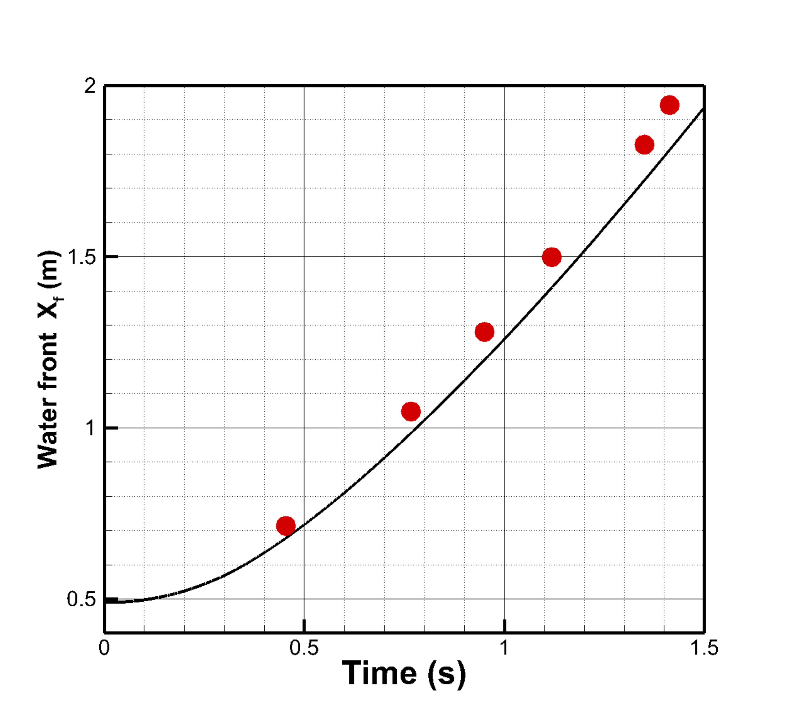
Fig. 13 presents a comparison of the water front calculated using ExaGOOP and the experimentally obtained water front values [3] at various times. The solid line indicates the ExaGOOP solution and the red circles denote the experimental data from [3]. A strong correlation is observed between the numerical and experimental values, thereby validating the solver.
(a) t = 0.0 s
(b) t = 0.15 s
(c) t = 0.22 s
(d) t = 0.29 s
Fig. 12 Evolution of water front in the 2-D dam break test case
(a)
Fig. 13 Comparison of the water front location with time. Solid line shows ExaGOOP solution and red circles indicate experimental data from [3]
Torsion of a three-dimensional elastic column
This test case verifies the UDF Moving Wall Boundary Conditions feature by twisting a linearly elastic column about its axis using a rotating top wall and comparing the resulting twist-angle profile against the analytical quasi-static solution.
Problem configuration
A square-cross-section elastic column occupies the domain \([-W, W]^2 \times [0, L]\) with half-width \(W = 0.25\) m and height \(L = 2\) m. The background nodal grid spans \([-B, B]^2 \times [0, L]\) with \(B = 0.6\) m and is discretised into \(12 \times 12 \times 20\) cells. Material properties are \(E = 10^7\) Pa, \(\nu = 0.3\), and \(\rho = 1000\) kg/m³.
Boundary conditions are:
Bottom face (\(z = 0\)): no-slip, zero velocity — clamped base.
Lateral faces (\(x = \pm B\), \(y = \pm B\)): slip walls.
Top face (\(z = L\)): no-slip with a UDF imposing solid-body rotation about the \(z\)-axis at angular velocity \(\omega = 0.5\) rad/s:
\[v_x = -\omega y, \qquad v_y = \omega x, \qquad v_z = 0.\]
The UDF is provided as a compiled shared library (libwall_twist). The
relevant input file lines are:
mpm.bc_zlo_mom            = noslip
mpm.bc_zhi_mom            = noslip
mpm.bc_zhi_mom.udf_lib    = "./UDF/libwall_twist.dylib"
mpm.bc_zhi_mom.udf_func   = "wall_vel_twist"
Analytical solution
Under quasi-static loading the twist angle grows linearly with height and linearly with time. For an elastic column driven by a rotating top wall, the expected twist angle at height \(z\) and time \(t\) is:
At \(z = 0\) the angle is zero (clamped base) and at \(z = L\) the angle equals \(\omega t\) (enforced by the wall).
ExaGOOP results
The MPM simulation is run to \(t = 4\) s using \(\text{CFL} = 0.3\) and the USL stress-update scheme with \(2^3 = 8\) material points per cell, giving 4000 material points in total.
Fig. 14 shows the twist-angle profile \(\theta(z)\) at a representative time snapshot compared to the analytical linear profile. The base (\(z = 0\)) remains fixed and the angle grows linearly towards the top, in close agreement with the analytical prediction.
Fig. 14 Twist-angle profile \(\theta(z)\) at a representative time snapshot. Red markers show the MPM result (mean rotation angle per horizontal layer); dashed line shows the analytical solution \(\theta = \omega t z / L\).
The test case is located in Tests/3D_Twisted_Column/. Pre-processing
and post-processing scripts are provided in the PreProcess/ and
PostProcess/ subdirectories respectively. The UDF source and
platform-aware Makefile are in UDF/.