Parametric & Sensitivity Analysis

SDOM’s ParametricStudy class lets you run a multi-dimensional sensitivity study with a single Python script. You define which parameters to vary and over what values, and SDOM automatically generates every combination (Cartesian product), solves each one in a separate worker process, and writes per-case CSV outputs plus a consolidated summary.

When to use parametric analysis

The table below maps the most common analysis needs to the sweep type that implements them. Each sweep type is documented in detail in the Sweep types section below.

Use case	Recommended approach	Typical parameters / inputs
Single scenario	`run_solver()` directly	—
Sensitivity on a scalar input	`ParametricStudy` + Scalar sweep (`add_scalar_sweep`)	Any row of `data["scalars"]` — e.g. `GenMix_Target`, `r` (discount rate), `LifeTimeVRE`, `EUE_max`, `AlphaNuclear`, `AlphaLargHy`, `AlphaOtheRe`
Sensitivity on storage costs or performance (uniform across all storage technologies)	`ParametricStudy` + Storage factor sweep (`add_storage_factor_sweep`)	Any row of `data["storage_data"]` — e.g. `P_Capex`, `E_Capex`, `Eff`, `FOM`, `VOM`, `Lifetime`, `Min_Duration`, `Max_Duration`
Sensitivity on a time-series profile (load growth, hydro availability, import/export limits or prices)	`ParametricStudy` + Time-series sweep (`add_ts_sweep`)	`load_data`, `large_hydro_data`, `large_hydro_max`, `large_hydro_min`, `cap_imports`, `price_imports`, `cap_exports`, `price_exports`
Full sensitivity across multiple parameters	`ParametricStudy` combining several of the sweep types above (every Cartesian combination is evaluated)	Any combination of the rows above

Quick-start example

Important

Windows users: Every script that calls study.run() must guard its entry point with if __name__ == "__main__":. On Windows, Python spawns child processes by re-importing the main script; without this guard the script recurses infinitely. This is a standard Python requirement — see Safe importing of main module.

The input data for this example is available in Data/no_exchange_run_of_river/ and pre-generated results (CSV files and figures) are stored under Data/no_exchange_run_of_river/results/.

import logging
import os

from sdom import configure_logging, get_default_solver_config_dict, load_data
from sdom.parametric import ParametricStudy
from sdom.analytic_tools import plot_parametric_results


def main():
    configure_logging(level=logging.INFO)

    # ── Load data ─────────────────────────────────────────────────────────────
    data_dir   = "./Data/no_exchange_run_of_river/"
    output_dir = "./Data/no_exchange_run_of_river/results/"

    data       = load_data(data_dir)
    solver_cfg = get_default_solver_config_dict(solver_name="highs", executable_path="")

    # ── Build study ───────────────────────────────────────────────────────────
    study = ParametricStudy(
        base_data=data,
        solver_config=solver_cfg,
        n_hours=96,
        output_dir=output_dir,
        n_cores=3,
    )

    # Sweep 1 — GenMix_Target scalar (carbon-free target)
    study.add_scalar_sweep("scalars", "GenMix_Target", [0.0, 0.8, 1.0])

    # Sweep 2 — Storage power CAPEX factor (all technologies scaled uniformly)
    study.add_storage_factor_sweep("P_Capex", [1.0, 0.7])

    # Sweep 3 — Load/demand scaling
    study.add_ts_sweep("load_data", [1.0, 1.4])

    # ── Run — 3 × 2 × 2 = 12 cases in parallel ───────────────────────────────
    results = study.run()

    # ── Plot cross-case comparisons + per-case figures ────────────────────────
    plot_parametric_results(
        study,
        results,
        group_by=["GenMix_Target", "P_Capex"],   # x-axis clusters
        hue_by="load_data",                       # bars within each cluster
        max_cases_per_figure=36,
        plot_per_case=True,
    )

    # ── Console summary ───────────────────────────────────────────────────────
    successful = [r for r in results if r.is_optimal]
    failed     = [r for r in results if not r.is_optimal]
    print(f"Total: {len(results)}  |  Optimal: {len(successful)}  |  Failed: {len(failed)}")
    for r in successful:
        print(f"  cost={r.total_cost:>15,.0f}  status={r.solver_status}")


if __name__ == "__main__":
    main()

Sample results of this example

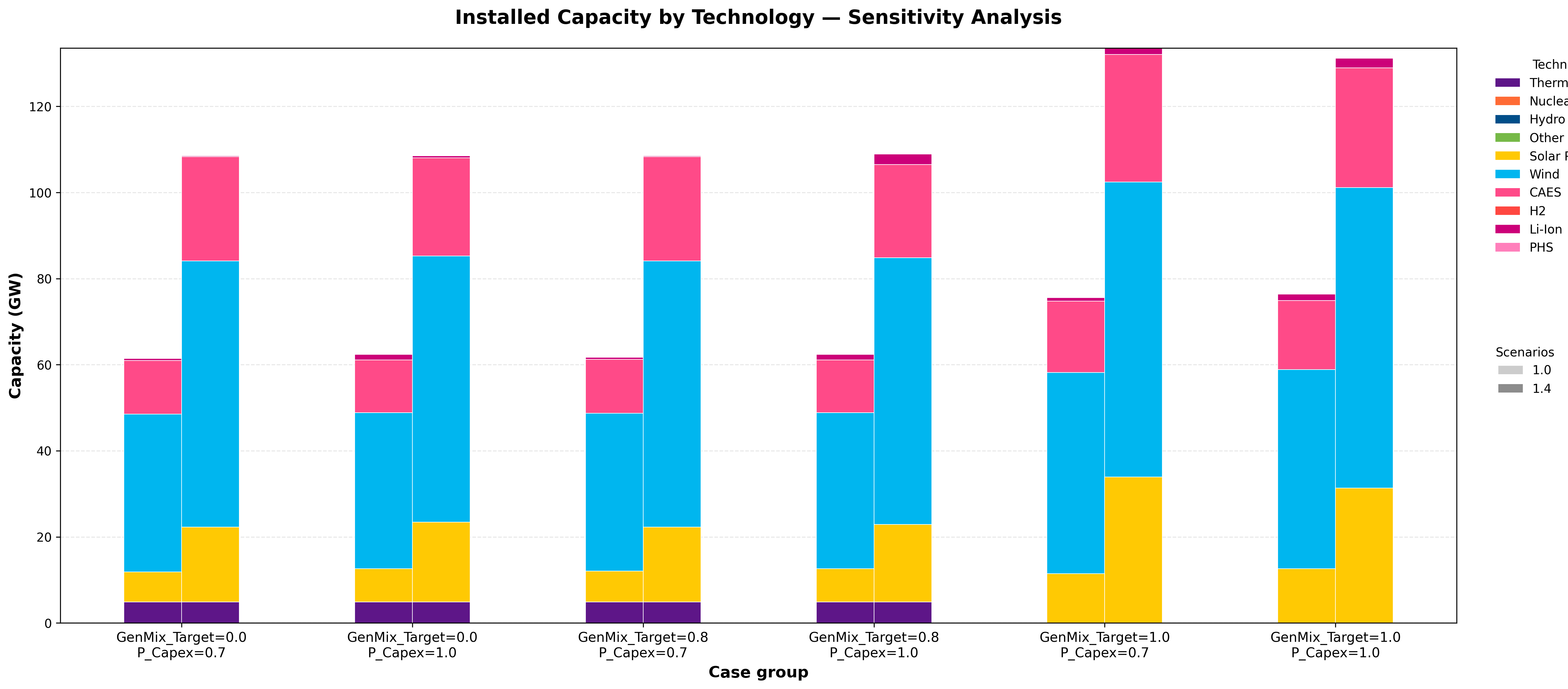
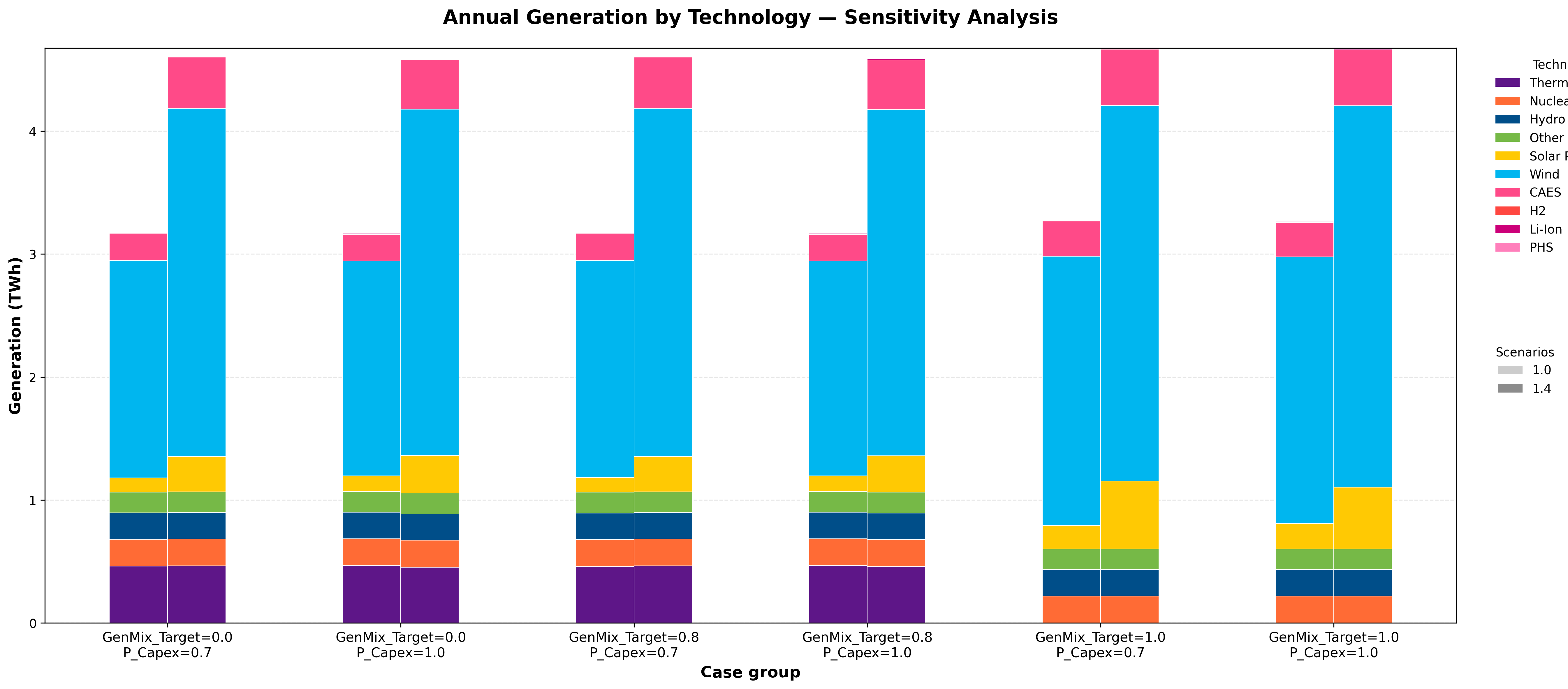
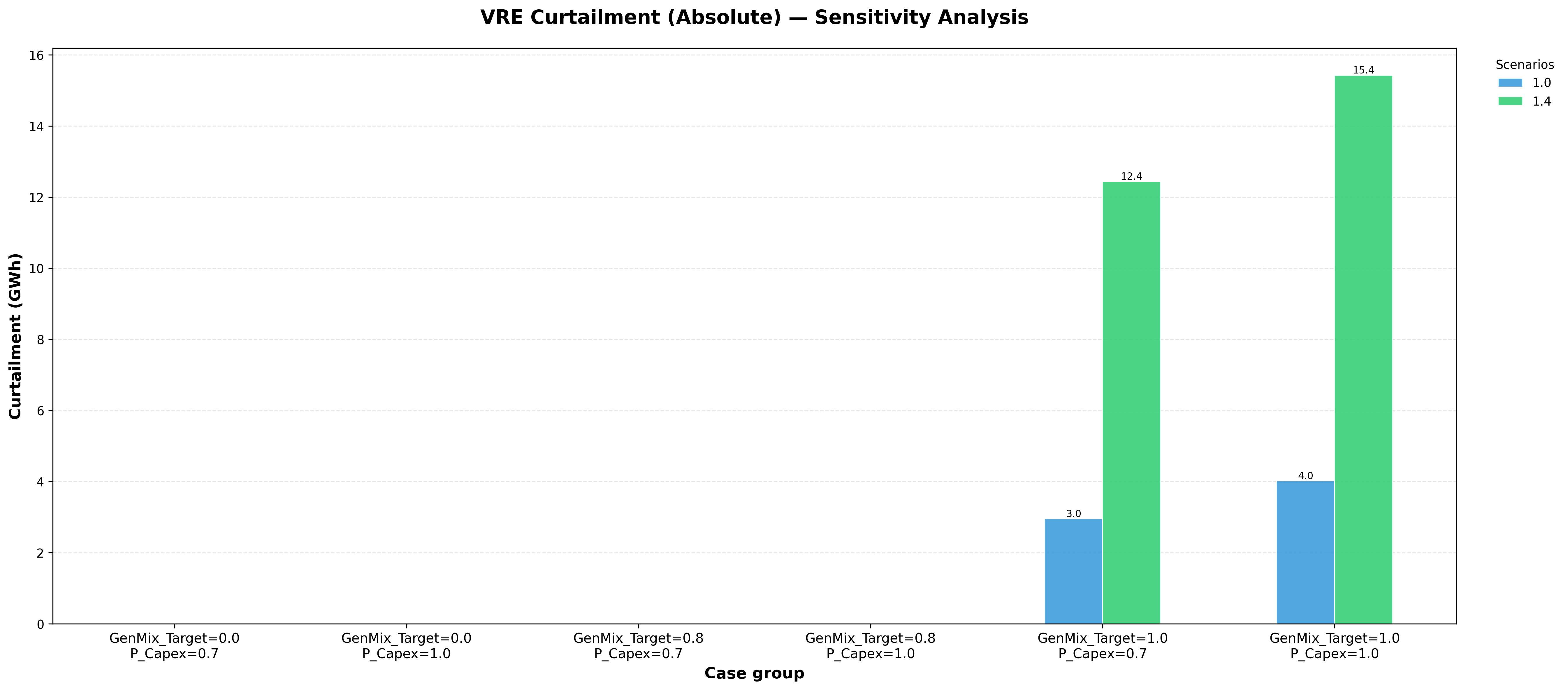
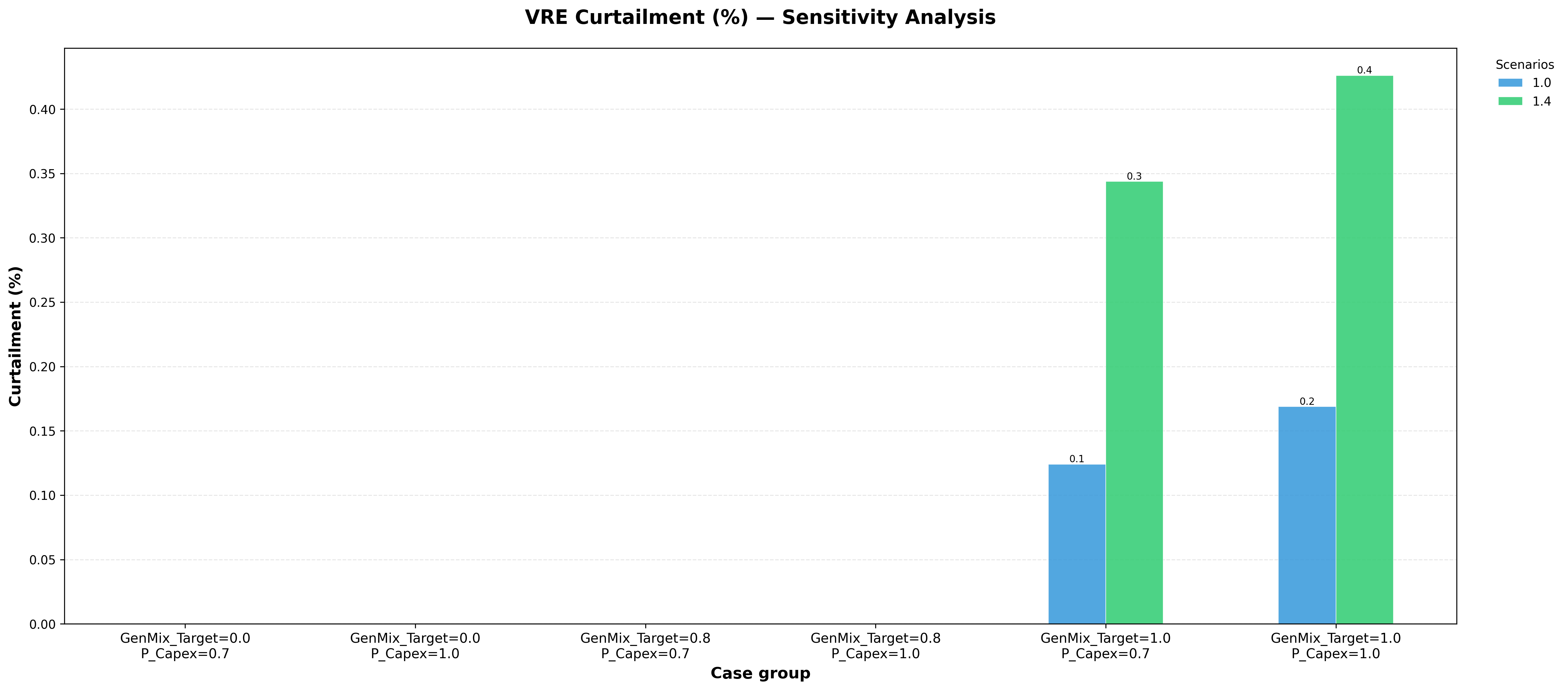
The figures below are the actual outputs obtained by running the example above (12 cases: GenMix_Target × 3, P_Capex × 2, load × 2).

Cross-case sensitivity plots

Installed capacity by technology

Capacity comparison

Total generation by technology

Generation comparison

VRE curtailment (absolute, MWh)

Curtailment — absolute

VRE curtailment (percentage)

Curtailment — percentage

Per-case plots

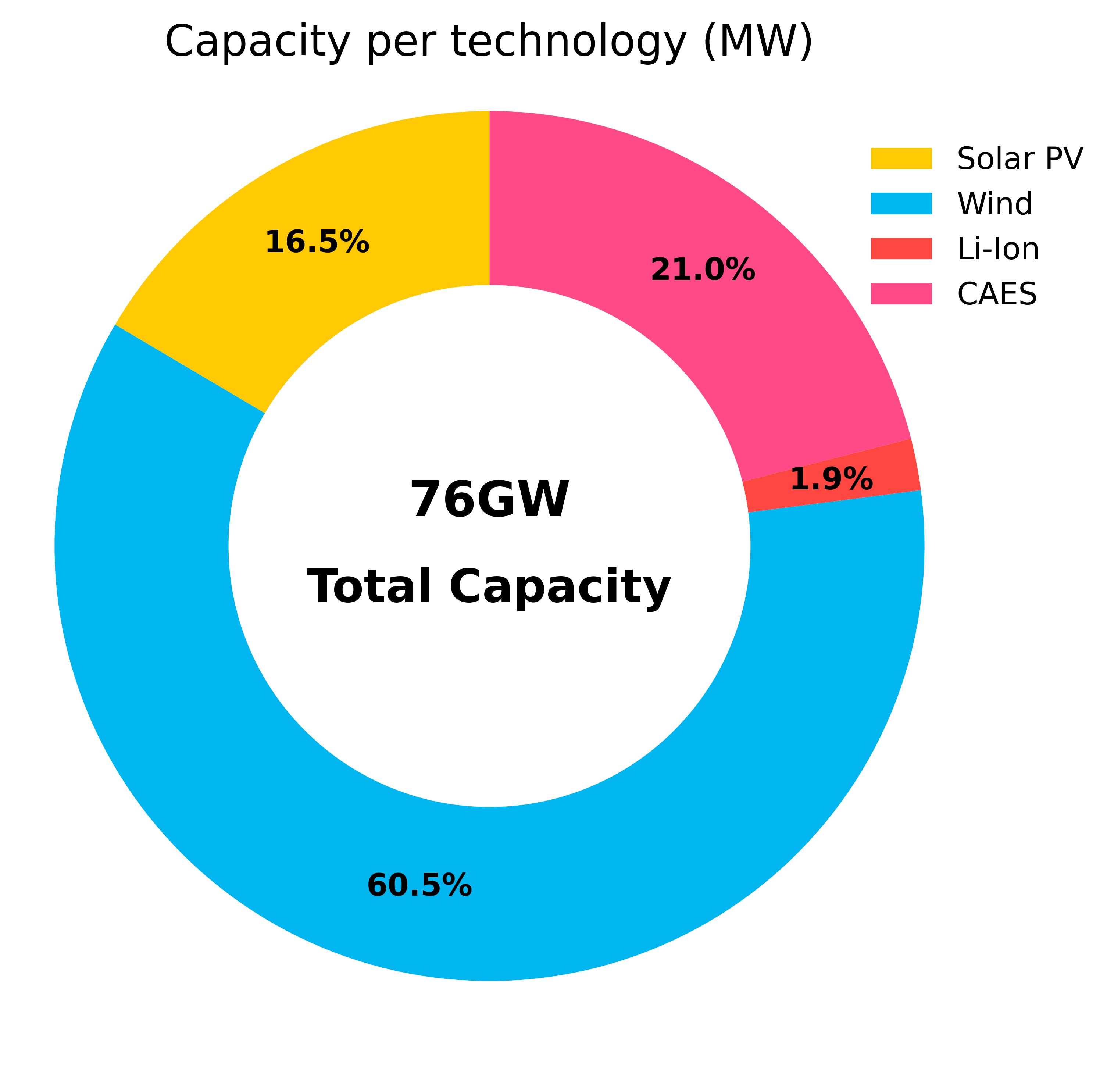
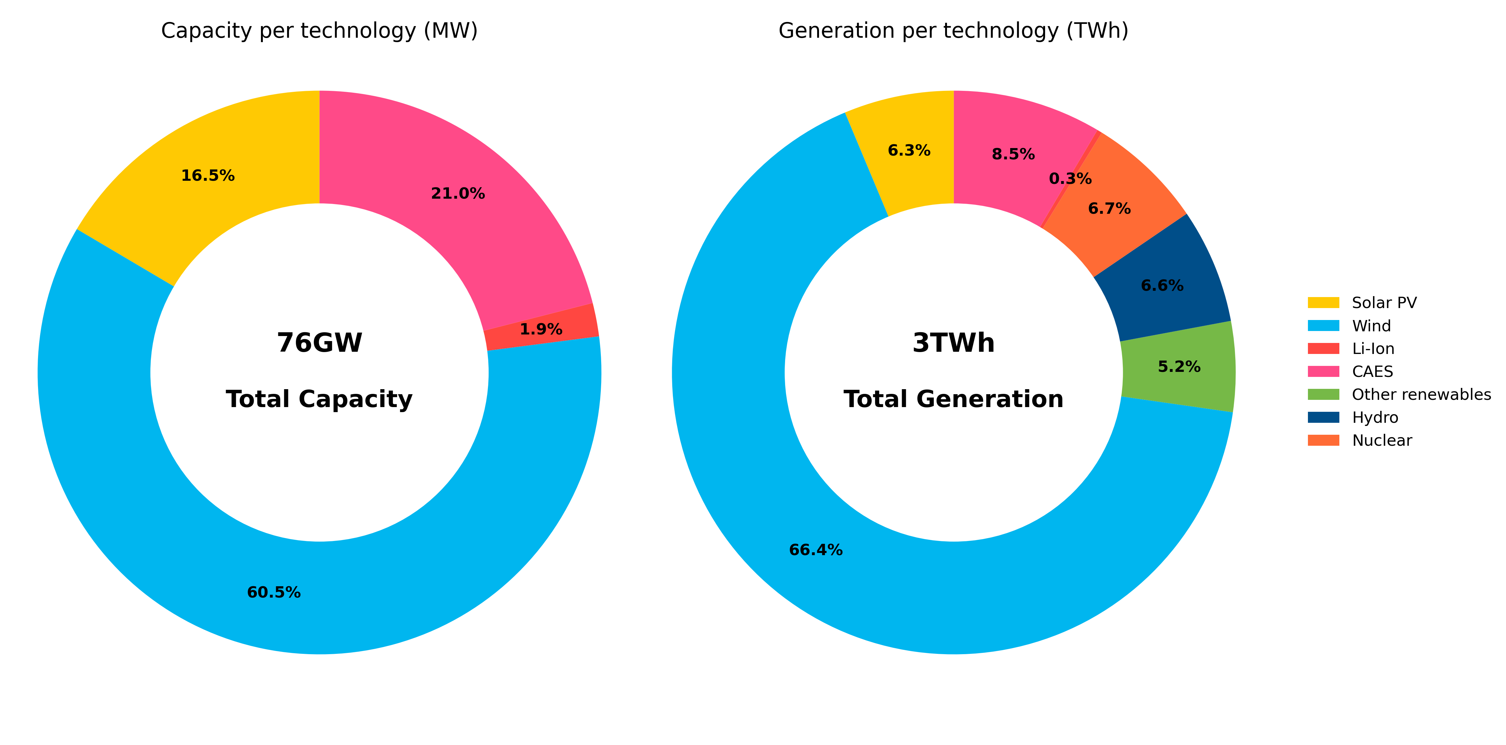
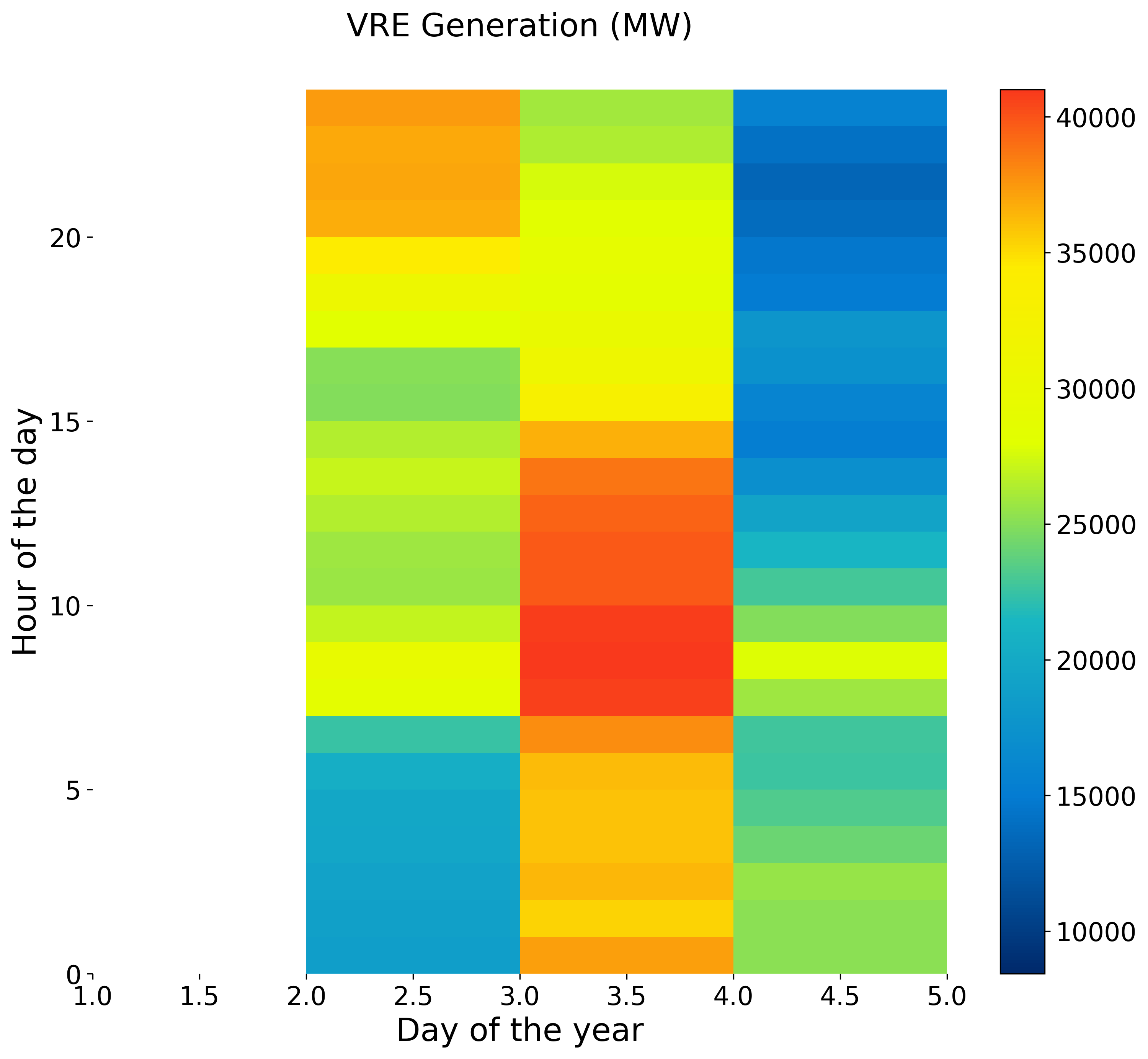
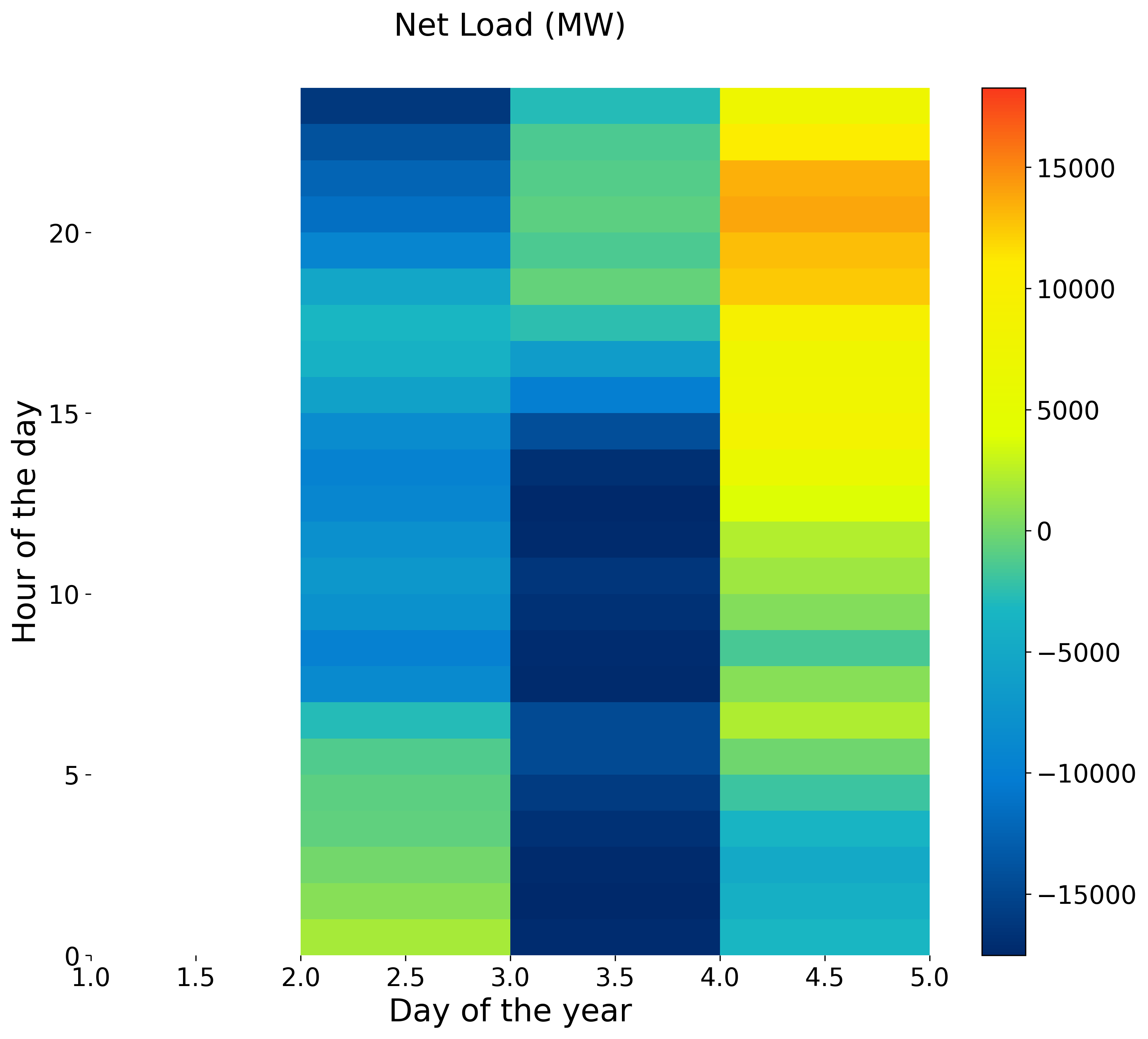
For each optimal case, individual figures are generated. The sample below is from case GenMix_Target=1.0 | P_Capex×1.0 | load×1.0.

Installed capacity donut

Capacity donut

Capacity and generation donuts (side by side)

Capacity and generation donuts

Hourly dispatch heatmap — VRE generation

Heatmap — VRE generation

Hourly dispatch heatmap — net load

Heatmap — net load

Sweep types

Scalar sweep — `add_scalar_sweep(data_key, param_name, values)`

Replaces a single entry in a row-indexed DataFrame with discrete absolute values.

# data["scalars"].loc["GenMix_Target", "Value"] → 0.7, 0.8, …
study.add_scalar_sweep("scalars", "GenMix_Target", [0.7, 0.8, 0.9, 1.0])

Storage factor sweep — `add_storage_factor_sweep(param_name, factors)`

Multiplies the entire data["storage_data"].loc[param_name] row (all storage technologies) by each factor uniformly.

# data["storage_data"].loc["P_Capex"] *= 0.7  /  *= 0.8  /  *= 1.0
study.add_storage_factor_sweep("P_Capex", [0.7, 0.8, 1.0])

Time-series sweep — `add_ts_sweep(ts_key, factors)`

Multiplies the numeric column of a time-series DataFrame by each factor. The column name is resolved automatically:

`ts_key`	Column scaled
`"load_data"`	`"Load"`
`"large_hydro_data"`	`"LargeHydro"`
`"large_hydro_max"`	`"LargeHydro_max"`
`"large_hydro_min"`	`"LargeHydro_min"`
`"cap_imports"`	`"Imports"`
`"price_imports"`	`"Imports_price"`
`"cap_exports"`	`"Exports"`
`"price_exports"`	`"Exports_price"`

study.add_ts_sweep("load_data", [0.9, 1.0, 1.1])
study.add_ts_sweep("large_hydro_max", [0.8, 1.0])

Cartesian product and case naming

Every combination of all registered sweeps is evaluated. A study with 3 scalar values, 2 storage factors, and 3 load factors produces 3 × 2 × 3 = 18 cases.

Each case receives a deterministic, filesystem-safe name derived from its parameter values, for example:

GenMix_Target=0.90_P_Capexx0.8_load_datax1.05

This name is used as the case_name in run_solver and as the sub-directory name under output_dir.

Note

If two combinations happen to produce the same safe name after character substitution (e.g. both 1.0/2 and 1.0_2 collapse to 1.0_2), SDOM automatically appends the case’s Cartesian-product index as a suffix (<name>_<index>) so every case directory is always unique.

Output structure

Running the example above produces the following layout under output_dir:

Data/no_exchange_run_of_river/results/
├── GenMix_Target=0.0_P_Capexx0.7_load_datax1.0/
│   ├── OutputGeneration_<case_name>.csv
│   ├── OutputStorage_<case_name>.csv
│   ├── OutputSummary_<case_name>.csv
│   ├── OutputThermalGeneration_<case_name>.csv
│   ├── OutputInstalledPowerPlants_<case_name>.csv
│   └── plots/
│       ├── capacity_donut.png
│       ├── capacity_generation_donuts.png
│       ├── heatmap_VRE_Generation_(MW).png
│       ├── heatmap_All_Thermal_Generation_(MW).png
│       ├── heatmap_Hydro_Generation_(MW).png
│       ├── heatmap_Nuclear_Generation_(MW).png
│       ├── heatmap_Other_Renewables_Generation_(MW).png
│       ├── heatmap_Storage_Charge_Discharge_(MW).png
│       ├── heatmap_Load_(MW).png
│       └── heatmap_Net_Load_(MW).png
├── GenMix_Target=0.0_P_Capexx0.7_load_datax1.4/
│   └── ...                                        # same structure, 11 more cases
├── ...
├── sensitivity_plots/
│   ├── capacity_comparison.png
│   ├── generation_comparison.png
│   ├── curtailment_absolute.png
│   ├── curtailment_percentage.png
│   └── cost_comparison.png
└── parametric_summary.csv

parametric_summary.csv has one row per case and always includes:

Column	Description
`case_name`	Unique identifier
`<data_key>.<param_name>`	Value used for each scalar sweep
`storage_data.<param>_factor`	Factor used for each storage sweep
`<ts_key>_factor`	Factor used for each ts sweep
`is_optimal`	`True` if the solver found an optimal solution
`total_cost`	Objective value (USD)
`solver_status`	Solver status string
`termination_condition`	Solver termination condition

Performance guidance

n_cores — Each worker process builds its own Pyomo model and runs the solver independently. Memory consumption scales roughly linearly with the number of concurrent workers — not with the total sweep size — because each worker deep-copies the base data inside its own process (lazy copy), so the parent process holds only one copy of the data at all times. A safe starting point is 4 workers; increase only if memory usage is comfortable. Pass n_cores=None to use all available cores minus one.
Large sweeps — For 50+ cases, consider whether output_dir is on a fast local disk; solver log files (HiGHS/CBC) are written per process and may create I/O contention on networked drives.
n_hours=72 for debugging — Use a short horizon to verify sweep logic and case naming before committing to a full 8760-hour run.
Failed cases — ParametricStudy.run() never raises on individual case failures. Inspect result.is_optimal and result.termination_condition per result, and check parametric_summary.csv for a consolidated view. Failed cases have total_cost=NaN in the summary so they are distinguishable from valid zero-cost results.

Visualising parametric results

After calling study.run(), use plot_parametric_results() from the analytic_tools sub-package to automatically produce:

Per-case plots — capacity donut, capacity + generation donuts, and hourly dispatch heatmaps for every optimal case, saved under <output_dir>/<case_name>/plots/.

Cross-case comparison plots — grouped stacked-bar charts for installed capacity, total generation, VRE curtailment, and CAPEX + OPEX costs by technology, saved under <output_dir>/sensitivity_plots/.

File	Description
`capacity_comparison.png`	Installed capacity by technology (GW)
`generation_comparison.png`	Annual generation by technology (TWh)
`curtailment_absolute.png`	VRE curtailment in absolute terms (GWh)
`curtailment_percentage.png`	VRE curtailment as percentage of total generation
`cost_comparison.png`	CAPEX (solid) and OPEX (hatched) by technology ($M USD)

The call used in the example script is:

plot_parametric_results(
    study,
    results,
    group_by=["GenMix_Target", "P_Capex"],   # x-axis clusters
    hue_by="load_data",                       # bars colour-coded by load factor
    max_cases_per_figure=36,
    plot_per_case=True,
)

Grouping strategy

Use group_by, hue_by, and facet_by to control how cases are arranged. Pass the same name that was registered with the sweep methods.

Parameter	Role
`group_by`	X-axis clusters — one cluster per unique combination of values (required)
`hue_by`	Bars within each cluster, colour-coded by this dimension (optional)
`facet_by`	One complete figure per unique value of this dimension (optional)

Tip

Dimension names must match exactly the names registered with the sweep methods. Use study.case_metadata[0].keys() to inspect available names after a run.

Additional options

Skip per-case plots (faster for large sweeps):

plot_parametric_results(study, results, group_by="GenMix_Target", plot_per_case=False)

Override the output directory:

plot_parametric_results(study, results, group_by="GenMix_Target",
                        output_dir="./my_output/")

Limit cases per figure (auto-splits into part1.png, part2.png, …):

plot_parametric_results(study, results, group_by="GenMix_Target",
                        max_cases_per_figure=12)

Faceted figures (one complete figure per load factor):

plot_parametric_results(
    study, results,
    group_by="GenMix_Target",
    hue_by="P_Capex",
    facet_by="load_data",
)