Transmission Line Loading and Utilization

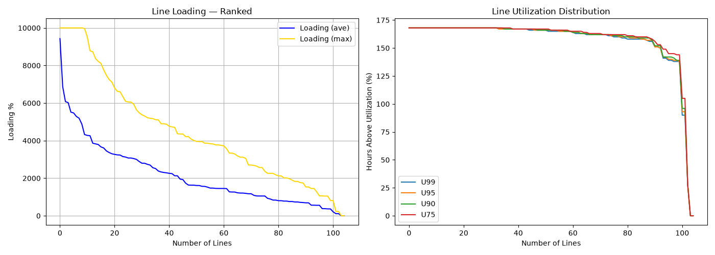
Two transmission views:

1. Loading ranked — line loading (% of rating) sorted descending, showing which lines hit the highest utilization across the horizon.

2. Utilization — distribution of hours each line operates above threshold percentiles (90/95/99% of rating).

The Sienna RTS-GMLC fixture is solved with DCPPowerModel, so the simulation store carries FlowActivePowerVariable__Line data and these plots work out of the box. The same calls work against a Plexos scenario (PlexosScenario(simulation_files=...)) — the transmission API is shared across scenario types.

/home/runner/work/GridAnalysisToolkit/GridAnalysisToolkit/src/gat/datahelpers/sienna.py:381: UserWarning: StandardLoad was not found. Use one of the following components
  warnings.warn(message, UserWarning)
----- Available Components -----
RenewableNonDispatch
LoadZone
RenewableDispatch
FixedAdmittance
ACBus
Area
VariableReserve
TwoTerminalHVDCLine
ThermalStandard
Arc
PowerLoad
TapTransformer
Line
calculating loading
calculating loading
formatting dataframe

import warnings

warnings.filterwarnings("ignore", category=DeprecationWarning)

import matplotlib.pyplot as plt

from gat.scenariohandlers import SiennaScenario
import gat.quickplots as qp

# These examples use the in-repo Sienna RTS-GMLC fixture. Regenerate it via
# `make sienna-fixture-v4`. For project-based workflows, use `gat.load(...)`
# instead — see docs/source/python_api_load.md.
sienna_v4 = "../../example_data/sienna/v4"
scenario = SiennaScenario(
    simulation_files=f"{sienna_v4}/simulation_store.h5",
    system_file=f"{sienna_v4}/sys.json",
)

loading = scenario.get_line_loading()
utilization = scenario.get_line_utilization()

fig, axs = plt.subplots(1, 2, figsize=(14, 5))

qp.plot_loading_ranked(loading, ax=axs[0])
axs[0].set_title("Line Loading — Ranked")

qp.plot_lines_utilization(utilization, ax=axs[1])
axs[1].set_title("Line Utilization Distribution")

plt.tight_layout()
plt.show()