PySAM for a Single Location

Run a PySAM pvsamv1 simulation for a single location, inspect the model output dictionary, and visualize the spatial rear-side ground irradiance profile beneath a bifacial array.

This notebook uses a cached NSRDB weather file for New York City that ships with the repository, so it runs fully offline with no API key or network access required.

import os
import json

import numpy as np
import pandas as pd
import matplotlib.pyplot as plt

import pvdeg
from pvdeg import DATA_DIR

# Load cached NSRDB weather for New York City, shipped with the pvdeg package.
# Reproducible and fully offline (no API key or network), and resolves from a pip
# install as well as a repo clone.
weather_path = os.path.join(DATA_DIR, "psm4_nyc.csv")
meta_path = os.path.join(DATA_DIR, "meta_nyc.json")

weather = pd.read_csv(weather_path, index_col=0, parse_dates=True)
with open(meta_path, "r") as f:
    meta = json.load(f)

meta

{'Source': 'NSRDB',
 'Location ID': '1245247',
 'City': '-',
 'State': '-',
 'Country': '-',
 'Clearsky DHI Units': 'w/m2',
 'Clearsky DNI Units': 'w/m2',
 'Clearsky GHI Units': 'w/m2',
 'Dew Point Units': 'c',
 'DHI Units': 'w/m2',
 'DNI Units': 'w/m2',
 'GHI Units': 'w/m2',
 'Solar Zenith Angle Units': 'Degree',
 'Temperature Units': 'c',
 'Pressure Units': 'mbar',
 'Relative Humidity Units': '%',
 'Precipitable Water Units': 'cm',
 'Wind Direction Units': 'Degrees',
 'Wind Speed Units': 'm/s',
 'Cloud Type -15': 'N/A',
 'Cloud Type 0': 'Clear',
 'Cloud Type 1': 'Probably Clear',
 'Cloud Type 2': 'Fog',
 'Cloud Type 3': 'Water',
 'Cloud Type 4': 'Super-Cooled Water',
 'Cloud Type 5': 'Mixed',
 'Cloud Type 6': 'Opaque Ice',
 'Cloud Type 7': 'Cirrus',
 'Cloud Type 8': 'Overlapping',
 'Cloud Type 9': 'Overshooting',
 'Cloud Type 10': 'Unknown',
 'Cloud Type 11': 'Dust',
 'Cloud Type 12': 'Smoke',
 'Fill Flag 0': 'N/A',
 'Fill Flag 1': 'Missing Image',
 'Fill Flag 2': 'Low Irradiance',
 'Fill Flag 3': 'Exceeds Clearsky',
 'Fill Flag 4': 'Missing CLoud Properties',
 'Fill Flag 5': 'Rayleigh Violation',
 'Surface Albedo Units': 'N/A',
 'Version': '4.1.2.dev4+g3b38bc8.d20250228',
 'latitude': 40.65,
 'longitude': -73.98,
 'altitude': 27,
 'tz': -5,
 'wind_height': 2}

out_dict = pvdeg.pysam.pysam(
    weather_df=weather,
    meta=meta,
    pv_model="pvsamv1",
    pv_model_default="FlatPlatePVCommercial",
)
for key in sorted(out_dict.keys()):
    print(key)

---------------------------------------------------------------------------
AttributeError                            Traceback (most recent call last)
Cell In[3], line 7
      3     meta=meta,
      4     pv_model="pvsamv1",
      5     pv_model_default="FlatPlatePVCommercial",
      6 )
----> 7 for key in sorted(out_dict.keys()):
      8     print(key)

AttributeError: 'NoneType' object has no attribute 'keys'

# Most outputs are scalars or 1-D time series. A few are 2-D matrices, returned
# as a tuple whose entries are themselves tuples (rows). Find those.
for key, item in out_dict.items():
    if isinstance(item, tuple) and item and isinstance(item[0], tuple):
        print(key)

annual_energy_distribution_time
subarray1_ground_rear_spatial
subarray1_poa_rear_spatial

Spatial ground irradiance

A few outputs describe irradiance that varies across the ground between module rows and are returned as 2-D matrices (a tuple of row tuples):

• subarray1_ground_rear_spatial — rear-side irradiance reaching the ground.

• subarray1_poa_rear_spatial — rear-side plane-of-array irradiance.

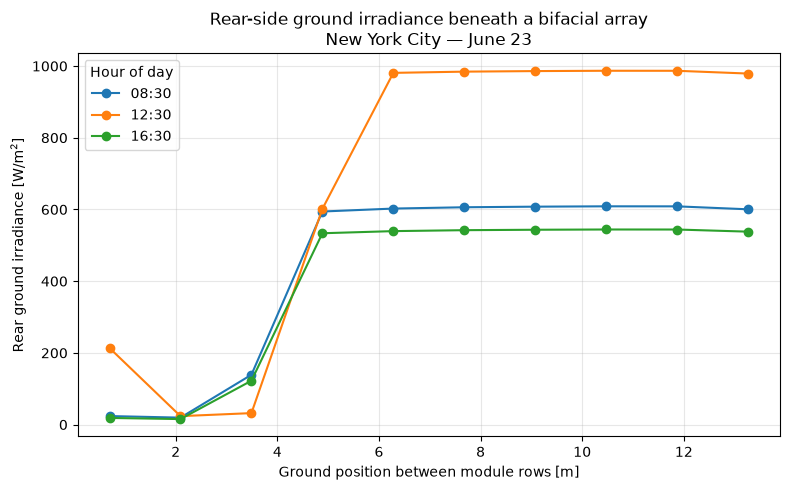
We visualize subarray1_ground_rear_spatial, which matters for agrivoltaics: it tells us how much light reaches the ground beneath a bifacial array. Its layout is:

• Row 0 — the ground positions (in metres) where irradiance is evaluated. The leading value is a 0 placeholder.

• Rows 1: — one row per hourly timestep. The leading value is the timestep index; the remaining values are the irradiance at each position.

spatial = out_dict["subarray1_ground_rear_spatial"]

# Row 0 holds the ground positions (drop the leading placeholder).
# In every data row, column 0 is the timestep index, so drop it too.
distances = np.array(spatial[0])[1:]
ground_irradiance = np.array(spatial[1:])[:, 1:]  # shape: (hours, positions)

# Pick the sunniest day (greatest total rear ground irradiance) to visualize.
daily_total = ground_irradiance.reshape(-1, 24, distances.size).sum(axis=(1, 2))
best_day = int(daily_total.argmax())

day_slice = slice(best_day * 24, best_day * 24 + 24)
day_index = weather.index[day_slice]
day_irradiance = ground_irradiance[day_slice]

# Ground irradiance varies across the pitch because the module rows cast a moving
# shadow. Plot the spatial profile at a few hours to see the shading band shift.
fig, ax = plt.subplots(figsize=(8, 5))

for hour in (8, 12, 16):
    ax.plot(
        distances,
        day_irradiance[hour],
        marker="o",
        label=day_index[hour].strftime("%H:%M"),
    )

ax.set_xlabel("Ground position between module rows [m]")
ax.set_ylabel("Rear ground irradiance [W/m$^2$]")
ax.set_title(
    "Rear-side ground irradiance beneath a bifacial array\n"
    f"New York City \u2014 {day_index[0].strftime('%B')} {day_index[0].day}"
)
ax.legend(title="Hour of day")
ax.grid(True, alpha=0.3)
fig.tight_layout()
plt.show()