Getting Started with FASTSim

This demo walks through the core FASTSim workflow: loading a vehicle, loading a drive cycle, running a simulation, and inspecting the results.

import os

import matplotlib.pyplot as plt

import fastsim as fsim

SHOW_PLOTS = os.environ.get("SHOW_PLOTS", "true").lower() == "true"

Setting Up a Simulation¶

Every FASTSim simulation needs three things: a Vehicle, a Cycle (the speed-vs-time trace the vehicle will attempt to follow), and a SimDrive that ties them together and runs the physics.

Loading a Vehicle¶

Vehicle.from_resource loads one of the sample vehicle YAML files bundled with FASTSim. Vehicle.list_resources() returns the full list of bundled vehicles (and Cycle.list_resources() does the same for drive cycles). The resource files themselves live in the fastsim-core resource directory. A few examples:

File	Type
`2012_Ford_Fusion.yaml`	Conventional
`2016_TOYOTA_Prius_Two.yaml`	Hybrid Electric (HEV)
`2022_Renault_Zoe_ZE50_R135.yaml`	Battery Electric (BEV)
`2020 Chevrolet Bolt EV thrml.yaml`	BEV with thermal model
`2021_Hyundai_Sonata_Hybrid_Blue_thrml.yaml`	HEV with thermal model

Vehicles with “thrml” in the filename include cabin, Heating, Ventilation, and Air Conditioning (HVAC), and battery thermal models. The non-thermal vehicles are simpler and are a good starting point.

veh = fsim.Vehicle.from_resource("2012_Ford_Fusion.yaml")

To use your own vehicle definition instead of a bundled one, load it from a YAML file on disk with Vehicle.from_file.

save_interval controls how often the vehicle records its internal state to history vectors. A value of 1 means every time step is recorded, which is what we need for per-step plotting. A larger value saves less frequently, and None disables history recording entirely. The bundled vehicles already default to a save_interval of 1, but we set it explicitly here to be clear about our intent.

veh.set_save_interval(1)

Loading a Drive Cycle¶

Cycle.from_resource loads a bundled drive cycle the same way. FASTSim ships with sample cycles including udds.csv (Urban Dynamometer Driving Schedule) and hwfet.csv (Highway Fuel Economy Test).

You can also load custom cycles from CSV files on disk with Cycle.from_file. A cycle CSV needs at minimum time_seconds and speed_meters_per_second columns.

cyc = fsim.Cycle.from_resource("udds.csv")

Running the Simulation¶

SimDrive takes a vehicle and a cycle and computes the vehicle’s powertrain response at each time step. Calling walk() runs the simulation from start to finish.

For a conventional vehicle, walk() runs through the cycle once. For hybrid vehicles, it iterates until the battery state of charge is balanced between the start and end of the cycle.

sd = fsim.SimDrive(veh, cyc)
sd.walk()

Inspecting Results¶

There are two main ways to get data out of a completed simulation:

to_dataframe() returns a Polars DataFrame (or pandas if you pass pandas=True) with one row per saved time step. Column names use dot-separated paths like veh.history.speed_ach_meters_per_second. This is the easiest way to plot time series.
to_pydict(flatten=True) serializes the full simulation state into a flat Python dictionary with the same dot-separated keys. This is useful for pulling out scalar values like total fuel energy consumed.

df = sd.to_dataframe(pandas=True)
sd_dict = sd.to_pydict(flatten=True)

print(f"Total fuel energy: {sd_dict['veh.pt_type.Conv.fc.state.energy_fuel_joules'] / 1e6:.2f} MJ")
print(f"Number of time steps: {len(df)}")
print(f"\nFirst 10 columns (of {len(df.columns)}):")
print(df.columns.tolist()[:10])

Total fuel energy: 26.29 MJ
Number of time steps: 1370

First 10 columns (of 62):
['veh.pt_type.Conv.fc.history.i', 'veh.pt_type.Conv.fc.history.pwr_out_max_watts', 'veh.pt_type.Conv.fc.history.pwr_prop_max_watts', 'veh.pt_type.Conv.fc.history.eff', 'veh.pt_type.Conv.fc.history.pwr_prop_watts', 'veh.pt_type.Conv.fc.history.energy_prop_joules', 'veh.pt_type.Conv.fc.history.pwr_aux_watts', 'veh.pt_type.Conv.fc.history.energy_aux_joules', 'veh.pt_type.Conv.fc.history.pwr_fuel_watts', 'veh.pt_type.Conv.fc.history.energy_fuel_joules']

Visualizing Results¶

Target vs. Achieved Speed¶

This plot compares the drive cycle’s target speed against what the vehicle actually achieved. For a vehicle with enough power to follow the trace, these two lines should overlap almost exactly.

fig, ax = plt.subplots(figsize=(10, 4))
ax.plot(
    df["cyc.time_seconds"],
    df["cyc.speed_meters_per_second"],
    label="Target",
    alpha=0.7,
)
ax.plot(
    df["cyc.time_seconds"],
    df["veh.history.speed_ach_meters_per_second"],
    label="Achieved",
    linestyle="--",
)
ax.set_xlabel("Time [s]")
ax.set_ylabel("Speed [m/s]")
ax.set_title("UDDS Drive Cycle: Target vs. Achieved Speed")
ax.legend()
plt.tight_layout()
if SHOW_PLOTS:
    plt.show()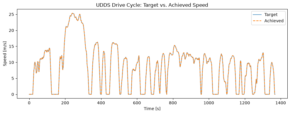

Fuel Converter Output Power¶

This plot shows the fuel converter’s total output power (propulsion plus auxiliary) over time. The 2012 Ford Fusion has a baseline auxiliary power of 700 W (pwr_aux_base_watts in the vehicle YAML).

fig, ax = plt.subplots(figsize=(10, 4))
ax.plot(
    df["cyc.time_seconds"],
    (
        df["veh.pt_type.Conv.fc.history.pwr_prop_watts"]
        + df["veh.pt_type.Conv.fc.history.pwr_aux_watts"]
    )
    / 1e3,
)
ax.set_xlabel("Time [s]")
ax.set_ylabel("FC Power [kW]")
ax.set_title("Fuel Converter Output Power")
plt.tight_layout()
if SHOW_PLOTS:
    plt.show()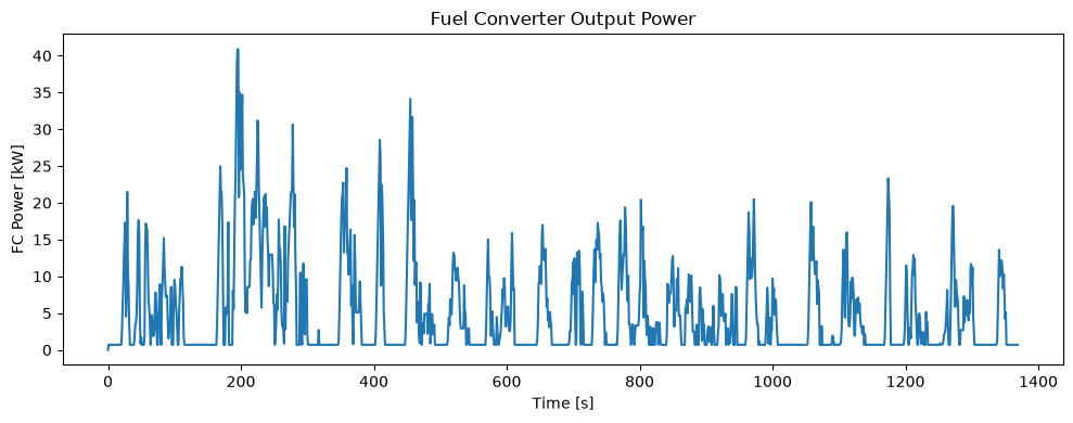

Cumulative Fuel Energy¶

Cumulative fuel energy consumed over the drive cycle.

fig, ax = plt.subplots(figsize=(10, 4))
ax.plot(
    df["cyc.time_seconds"],
    df["veh.pt_type.Conv.fc.history.energy_fuel_joules"] / 1e6,
)
ax.set_xlabel("Time [s]")
ax.set_ylabel("Cumulative Fuel Energy [MJ]")
ax.set_title("Cumulative Fuel Consumption")
plt.tight_layout()
if SHOW_PLOTS:
    plt.show()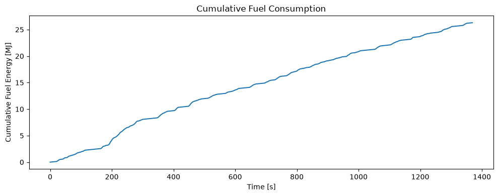

Source: fastsim/docs/demo_scripts/getting_started/demo_getting_started.py