Hybrid Electric Vehicle Demo

This demo simulates a Hybrid Electric Vehicle (HEV) over a drive cycle and visualizes the fuel converter, battery, and road load behavior.

import os
from pathlib import Path

import matplotlib.pyplot as plt
import seaborn as sns

import fastsim as fsim

sns.set_theme()

# if environment var `SHOW_PLOTS=false` is set, no plots are shown
SHOW_PLOTS = os.environ.get("SHOW_PLOTS", "true").lower() == "true"
# if environment var `SAVE_FIGS=true` is set, save plots
SAVE_FIGS = os.environ.get("SAVE_FIGS", "false").lower() == "true"

Setup and Simulation¶

Load a vehicle and drive cycle, configure per-step state recording, run the simulation, and extract the results.

# load 2016 Toyota Prius Two from file
veh = fsim.Vehicle.from_resource("2016_TOYOTA_Prius_Two.yaml")

# Set `save_interval` at vehicle level -- cascades to all sub-components with time-varying states
veh.set_save_interval(1)

# load cycle from file
cyc = fsim.Cycle.from_resource("udds.csv")

# instantiate `SimDrive` simulation object
sd = fsim.SimDrive(veh, cyc)
sd.walk()

df = sd.to_dataframe()
sd_dict = sd.to_pydict(flatten=True)

Visualize Results¶

The following plots show fuel converter, battery, and road load behavior over the drive cycle.

def plot_fc_pwr():
    """Plot fuel converter powers"""
    fig, ax = plt.subplots(3, 1, sharex=True, figsize=(10, 8))
    plt.suptitle("Fuel Converter Power")

    ax[0].plot(
        df["cyc.time_seconds"],
        (
            df["veh.pt_type.HEV.fc.history.pwr_prop_watts"]
            + df["veh.pt_type.HEV.fc.history.pwr_aux_watts"]
        )
        / 1e3,
        label="shaft",
    )
    ax[0].plot(
        df["cyc.time_seconds"],
        df["veh.pt_type.HEV.fc.history.pwr_fuel_watts"] / 1e3,
        label="fuel",
    )
    ax[0].set_ylabel("FC Power [kW]")
    ax[0].legend()

    ax[1].plot(
        df["cyc.time_seconds"],
        df["veh.pt_type.HEV.res.history.soc"],
    )
    ax[1].set_ylabel("SOC")

    ax[2].plot(
        df["cyc.time_seconds"],
        df["veh.history.speed_ach_meters_per_second"],
    )
    ax[2].set_xlabel("Time [s]")
    ax[2].set_ylabel("Ach Speed [m/s]")

    plt.tight_layout()
    if SAVE_FIGS:
        plt.savefig(Path("./plots/fc_pwr.svg"))
    if SHOW_PLOTS:
        plt.show()

    return fig, ax

Fuel converter output power (drivetrain + auxiliary) and fuel input power, with battery state of charge for context.

fig, ax = plot_fc_pwr()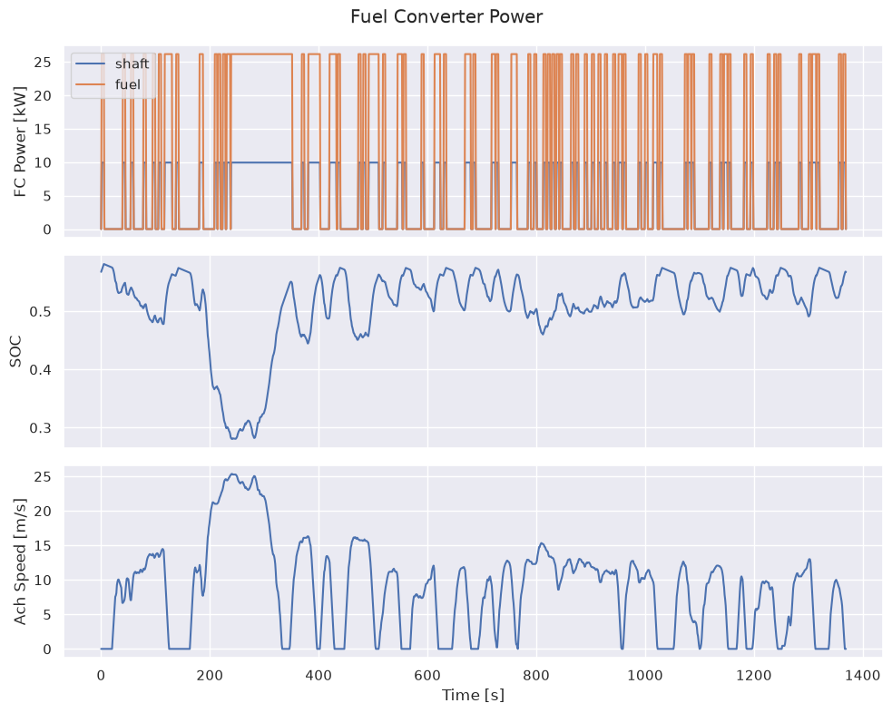

def plot_fc_energy():
    """Plot fuel converter energies"""
    fig, ax = plt.subplots(3, 1, sharex=True, figsize=(10, 8))
    plt.suptitle("Fuel Converter Energy")

    ax[0].plot(
        df["cyc.time_seconds"],
        (
            df["veh.pt_type.HEV.fc.history.energy_prop_joules"]
            + df["veh.pt_type.HEV.fc.history.energy_aux_joules"]
        )
        / 1e6,
        label="shaft",
    )
    ax[0].plot(
        df["cyc.time_seconds"],
        df["veh.pt_type.HEV.fc.history.energy_fuel_joules"] / 1e6,
        label="fuel",
    )
    ax[0].set_ylabel("FC Energy [MJ]")
    ax[0].legend()

    ax[1].plot(
        df["cyc.time_seconds"],
        df["veh.pt_type.HEV.res.history.soc"],
    )
    ax[1].set_ylabel("SOC")

    ax[2].plot(
        df["cyc.time_seconds"],
        df["veh.history.speed_ach_meters_per_second"],
    )
    ax[2].set_xlabel("Time [s]")
    ax[2].set_ylabel("Ach Speed [m/s]")

    plt.tight_layout()
    if SAVE_FIGS:
        plt.savefig(Path("./plots/fc_energy.svg"))
    if SHOW_PLOTS:
        plt.show()

    return fig, ax

Cumulative fuel converter output energy (drivetrain + auxiliary) and fuel input energy, with battery state of charge for context.

fig, ax = plot_fc_energy()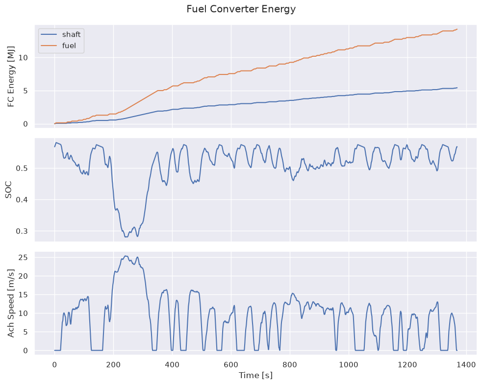

def plot_res_pwr():
    """Plot reversible energy storage powers"""
    fig, ax = plt.subplots(3, 1, sharex=True, figsize=(10, 8))
    plt.suptitle("Battery Power")

    ax[0].plot(
        df["cyc.time_seconds"],
        df["veh.pt_type.HEV.res.history.pwr_out_electrical_watts"] / 1e3,
        label="electrical out",
    )
    ax[0].plot(
        df["cyc.time_seconds"],
        df["veh.pt_type.HEV.res.history.pwr_out_chemical_watts"] / 1e3,
        label="chemical out",
    )
    ax[0].set_ylabel("RES Power [kW]")
    ax[0].legend()

    ax[1].plot(df["cyc.time_seconds"], df["veh.pt_type.HEV.res.history.soc"], label="soc")
    ax[1].plot(
        df["cyc.time_seconds"],
        df["veh.pt_type.HEV.res.history.soc_disch_buffer"],
        label="accel buffer",
        alpha=0.5,
    )
    ax[1].plot(
        df["cyc.time_seconds"],
        df["veh.pt_type.HEV.res.history.soc_regen_buffer"],
        label="regen buffer",
        alpha=0.5,
    )
    ax[1].axhline(sd_dict["veh.pt_type.HEV.res.min_soc"], color="blue", label="min soc")
    ax[1].axhline(sd_dict["veh.pt_type.HEV.res.max_soc"], color="red", label="max soc")
    ax[1].set_ylabel("SOC [-]")
    ax[1].legend(loc="center right")

    ax[2].plot(
        df["cyc.time_seconds"],
        df["veh.history.speed_ach_meters_per_second"],
    )
    ax[2].set_xlabel("Time [s]")
    ax[2].set_ylabel("Ach Speed [m/s]")

    plt.tight_layout()
    if SAVE_FIGS:
        plt.savefig(Path("./plots/battery_pwr.svg"))
    if SHOW_PLOTS:
        plt.show()

    return fig, ax

Battery electrical and chemical output power, with state of charge, discharge buffer, regen buffer, and min/max SOC limits.

fig, ax = plot_res_pwr()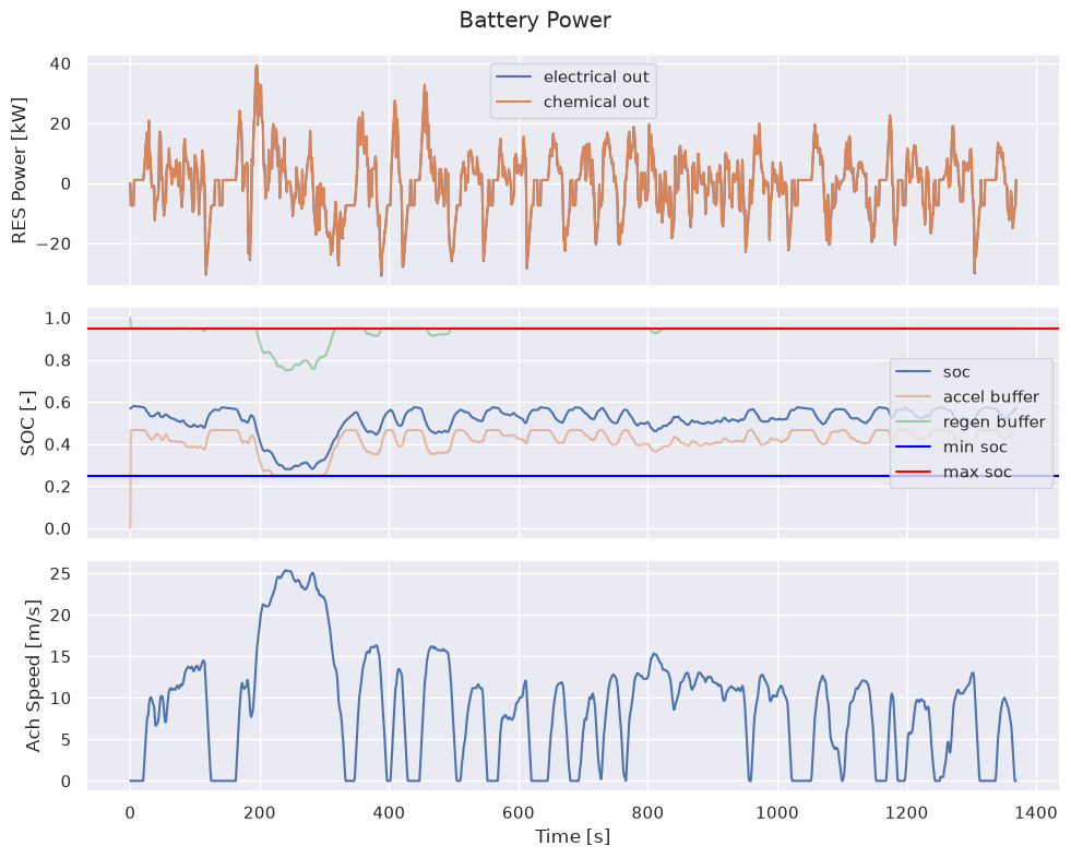

def plot_res_energy():
    """Plot reversible energy storage energies"""
    fig, ax = plt.subplots(3, 1, sharex=True, figsize=(10, 8))
    plt.suptitle("Battery Energy")

    ax[0].plot(
        df["cyc.time_seconds"],
        df["veh.pt_type.HEV.res.history.energy_out_electrical_joules"] / 1e6,
        label="electrical out",
    )
    ax[0].plot(
        df["cyc.time_seconds"],
        df["veh.pt_type.HEV.res.history.energy_out_chemical_joules"] / 1e6,
        label="chemical out",
    )
    ax[0].set_ylabel("RES Energy [MJ]")
    ax[0].legend()

    ax[1].plot(df["cyc.time_seconds"], df["veh.pt_type.HEV.res.history.soc"], label="soc")
    ax[1].plot(
        df["cyc.time_seconds"],
        df["veh.pt_type.HEV.res.history.soc_disch_buffer"],
        label="accel buffer",
        alpha=0.5,
    )
    ax[1].plot(
        df["cyc.time_seconds"],
        df["veh.pt_type.HEV.res.history.soc_regen_buffer"],
        label="regen buffer",
        alpha=0.5,
    )
    ax[1].set_ylabel("SOC [-]")
    ax[1].legend(loc="center right")

    ax[2].plot(
        df["cyc.time_seconds"],
        df["veh.history.speed_ach_meters_per_second"],
    )
    ax[2].set_xlabel("Time [s]")
    ax[2].set_ylabel("Ach Speed [m/s]")

    plt.tight_layout()
    if SAVE_FIGS:
        plt.savefig(Path("./plots/battery_energy.svg"))
    if SHOW_PLOTS:
        plt.show()

    return fig, ax

Cumulative battery electrical and chemical output energy, with state of charge and SOC buffers.

fig, ax = plot_res_energy()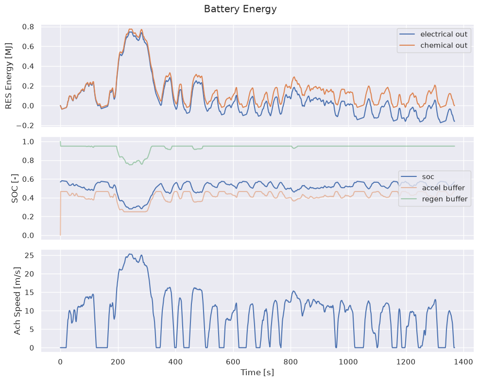

def plot_road_loads():
    """Plot road loads"""
    fig, ax = plt.subplots(2, 1, sharex=True, figsize=(10, 6))
    plt.suptitle("Road Loads")

    ax[0].plot(
        df["cyc.time_seconds"],
        df["veh.history.pwr_drag_watts"] / 1e3,
        label="drag",
    )
    ax[0].plot(
        df["cyc.time_seconds"],
        df["veh.history.pwr_rr_watts"] / 1e3,
        label="rolling resistance",
    )
    ax[0].set_ylabel("Power [kW]")
    ax[0].legend()

    ax[1].plot(
        df["cyc.time_seconds"],
        df["veh.history.speed_ach_meters_per_second"],
    )
    ax[1].set_xlabel("Time [s]")
    ax[1].set_ylabel("Ach. Speed [m/s]")

    plt.tight_layout()
    if SAVE_FIGS:
        plt.savefig(Path("./plots/road_loads.svg"))
    if SHOW_PLOTS:
        plt.show()

    return fig, ax

Aerodynamic drag power and rolling resistance power over the drive cycle.

fig, ax = plot_road_loads()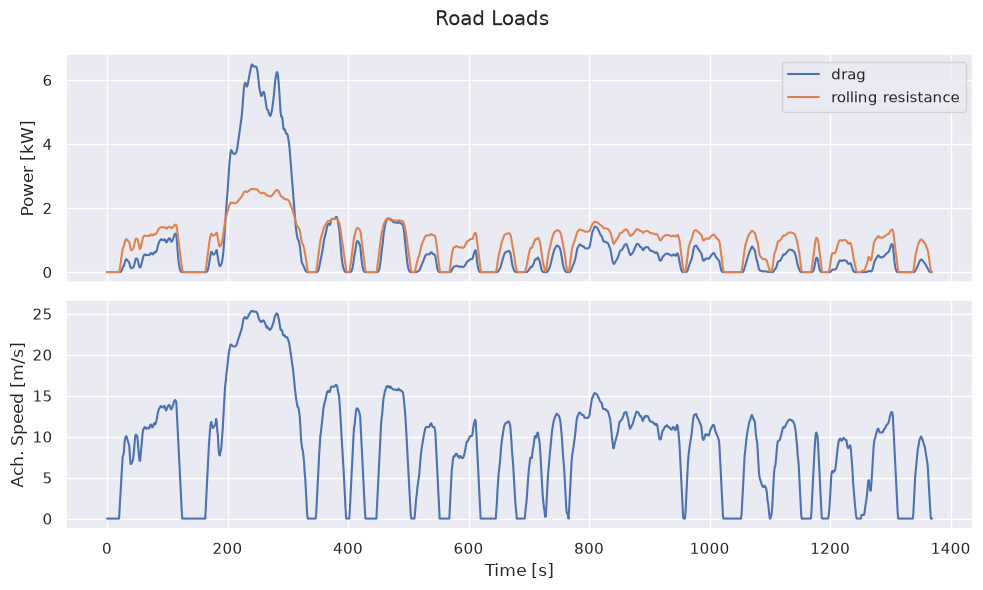

Source: fastsim/docs/demo_scripts/powertrains/demo_hev.py