How Filtration Works

gradeit() filters the elevation profile before it computes grade. By default, gradeit() uses Wood2014Filter. This is the five-step routine from Wood et al. (2014), Paper link.

See Methodology for more detail on the methodology.

import matplotlib.pyplot as plt
import numpy as np
from _data import TILE_DIR, load_coords

from gradeit import BridgeFilter, USGSLocal, gradeit

trace = load_coords("golden_creek")
elevation_model = USGSLocal(TILE_DIR)

# One palette for every figure on this page: the raw DEM is the neutral
# reference, the filtered profile carries the identity color, and red is
# reserved for what the filter is supposed to catch.
RAW = "#6b6b6b"
FILTERED = "#1f77b4"
BRIDGE = "#e06c00"
ARTIFACT = "#b3282d"

# Value labels sit on a scrap of the surface so a line never runs through them.
LABEL_BOX = {"facecolor": "white", "edgecolor": "none", "alpha": 0.85, "pad": 1.0}

Raw Elevation

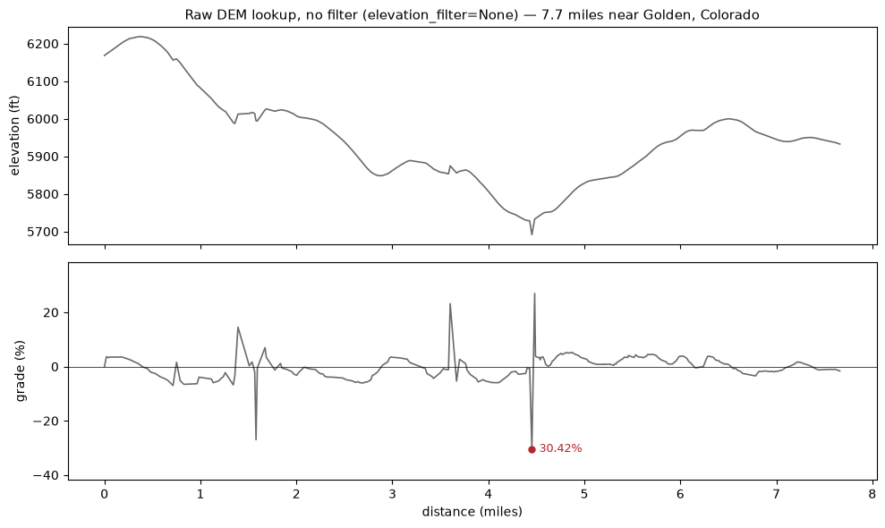
To start, we can look at just the raw elevation profile from our example trace in Golden, CO:

raw = gradeit(trace, elevation_model=elevation_model, elevation_filter=None)
miles = np.cumsum(raw.distances_ft) / 5280

fig, (ax_elev, ax_grade) = plt.subplots(2, 1, figsize=(10, 6), sharex=True)

ax_elev.plot(miles, raw.elevation_ft_unfiltered, color=RAW, lw=1.2)
ax_elev.set_ylabel("elevation (ft)")
ax_elev.set_title(
    "Raw DEM lookup, no filter (elevation_filter=None) — "
    f"{raw.distances_ft.sum() / 5280:.1f} miles near Golden, Colorado",
    fontsize=11,
)

raw_pct = 100 * raw.grade_dec_unfiltered
spike = int(np.argmax(np.abs(raw_pct)))
ax_grade.plot(miles, raw_pct, color=RAW, lw=1.2)
ax_grade.axhline(0, color="k", lw=0.5)
ax_grade.plot(miles[spike], raw_pct[spike], "o", ms=5, color=ARTIFACT)
ax_grade.annotate(
    f"  {abs(raw_pct[spike]):.2f}%",
    (miles[spike], raw_pct[spike]),
    fontsize=9,
    color=ARTIFACT,
    va="center",
)
ax_grade.set_ylabel("grade (%)")
ax_grade.set_xlabel("distance (miles)")
ax_grade.margins(y=0.2)

fig.tight_layout()
plt.show()

Bare Earth Artifacts

Next, let's look at a case where the DEM shows a artifact from using a bare-earth model. In this example, we'll zoom in on a section where the road crosses over the Clear Creek river around mile 4.5. The elevation that gets reported back to us shows the elevation drop down and then go back up. But, in reality, the road was constructed to go over the river and so the real grade is much less.

filtered = gradeit(trace, elevation_model=elevation_model)
creek = 119
assert np.argmax(np.abs(filtered.elevation_ft_filtered - raw.elevation_ft_unfiltered)) == creek

deck = (raw.elevation_ft_unfiltered[creek - 1] + raw.elevation_ft_unfiltered[creek + 1]) / 2
lo, hi = creek - 12, creek + 13
x = miles[lo:hi]

fig, (ax_elev, ax_grade) = plt.subplots(2, 1, figsize=(9, 6), sharex=True)

for ax, key, ylabel in ((ax_elev, "elev", "elevation (ft)"), (ax_grade, "grade", "grade (%)")):
    raw_y = raw.elevation_ft_unfiltered if key == "elev" else 100 * raw.grade_dec_unfiltered
    filt_y = (
        filtered.elevation_ft_filtered if key == "elev" else 100 * filtered.grade_dec_filtered
    )
    ax.plot(x, raw_y[lo:hi], color=RAW, lw=1.4, label="raw DEM")
    ax.plot(x, filt_y[lo:hi], color=FILTERED, lw=2.0, label="default filter")
    ax.axvline(miles[creek], color=ARTIFACT, lw=1.0, ls=":")
    ax.set_ylabel(ylabel)
    ax.margins(y=0.25)

for label, series, color, dy in (
    ("raw", raw.elevation_ft_unfiltered, RAW, -12),
    ("filtered", filtered.elevation_ft_filtered, FILTERED, 14),
):
    ax_elev.plot(miles[creek], series[creek], "o", ms=5, color=color)
    ax_elev.annotate(
        f"{label} {series[creek]:,.1f} ft ({series[creek] - deck:+.1f})",
        (miles[creek], series[creek]),
        textcoords="offset points",
        xytext=(10, dy),
        fontsize=8,
        color=color,
        bbox=LABEL_BOX,
    )

ax_grade.axhline(0, color="k", lw=0.5)
ax_grade.set_xlabel("distance (miles)")
ax_elev.legend(loc="upper right", fontsize=8)
ax_elev.set_title("The Clear Creek Crossing", fontsize=11)
fig.tight_layout()
plt.show()

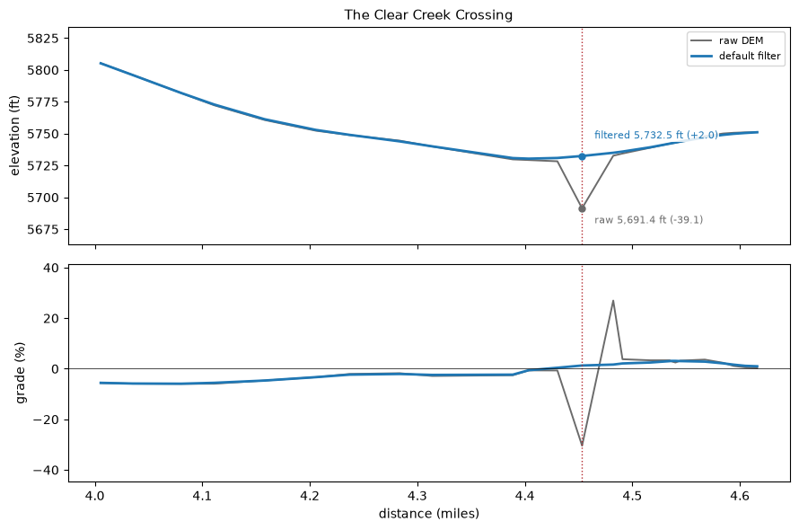
Notice how the filtered elevation profile correcly captures and corrects for this artifact.

A filter that is wrong for this trace

In addition to the default elevation filter, we also have a BridgeFilter that is used to detect and correct long bridge spans that the default filter can't catch. But, this filter can also catch real valleys where the road actually follows the terrain and so it should be used with caution. To show an example of that we can apply the bridge filter to our trace and see what happens.

over = gradeit(trace, elevation_model=elevation_model, elevation_filter=BridgeFilter())
delta = np.abs(over.elevation_ft_filtered - raw.elevation_ft_unfiltered)
touched = np.flatnonzero(delta > 1.0)

lo = max(touched.min() - 25, 0)
hi = min(touched.max() + 25, len(trace))
x = miles[lo:hi]
deepest = int(np.argmax(delta))

fig, ax = plt.subplots(figsize=(10, 4.4))
ax.axvspan(miles[touched.min()], miles[touched.max()], color=BRIDGE, alpha=0.12, lw=0)
ax.plot(x, raw.elevation_ft_unfiltered[lo:hi], color=RAW, lw=1.4, label="raw DEM")
ax.plot(
    x,
    filtered.elevation_ft_filtered[lo:hi],
    color=FILTERED,
    lw=1.6,
    label="Wood2014Filter (default)",
)
ax.plot(
    x,
    over.elevation_ft_filtered[lo:hi],
    color=BRIDGE,
    lw=2.0,
    ls="--",
    label="BridgeFilter() 1-mile default",
)
ax.annotate(
    "",
    xy=(miles[deepest], raw.elevation_ft_unfiltered[deepest]),
    xytext=(miles[deepest], over.elevation_ft_filtered[deepest]),
    arrowprops={"arrowstyle": "<->", "color": BRIDGE, "lw": 1.4},
)
ax.set_ylabel("elevation (ft)")
ax.set_xlabel("distance (miles)")
ax.set_title(
    "BridgeFilter incorrectly added a bridge over a real valley",
    fontsize=10,
)
ax.legend(loc="lower left", fontsize=8)
ax.margins(y=0.2)
fig.tight_layout()
plt.show()

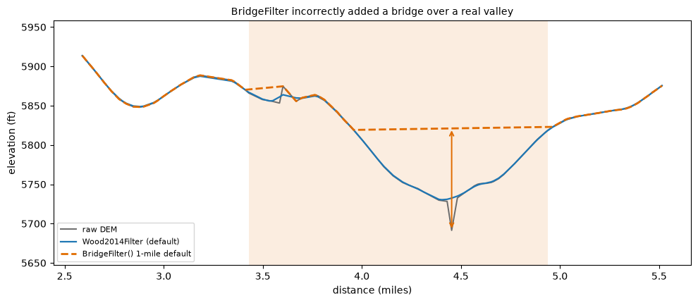
Note that the BridgeFilter incorrectly added a bridge over a real valley. It's not that BridgeFilter is broken. Bare-Earth Bridges shows a trace where BridgeFilter is the only filter that works. The lesson here is to make sure you're only using the BridgeFilter on traces where real large bridges are known to exist and that the baseline_radius_ft of the BridgeFilter is tuned to match the expected size of the crossing.