Model Prediction

RouteE models can be loaded from a large library of pre-trained models. Conventional gasoline (CV), hybrid electric (HEV), plug-in hybrid electric (PHEV), and battery electric (BEV) powertrain types are all available.

A note on PHEVs: Plug-in hybrids have two general operating modes 1) "Charge Depleting" or "EV" mode, where the vehicle relies only on energy from the battery to power the motor and 2) "Charge Sustaining" or "Hybrid" mode, where the vehicle operates like a typical parallel hybrid, using a combination of the combustion energy and electric motor for tractive effort and regenerative braking. Since the operating mode depends on battery state-of-charge and driver decisions, pre-trained RouteE-Powertrain models for both operating modes are provided for all PHEVs and it is up to the user to decide which is most appropriate for a particular application.

Picking a registry

By default, routee.powertrain fetches models from the public HuggingFace Hub catalog. For this example we'll use the small bundled registry that ships with the package so the notebook runs fully offline — set ROUTEE_REGISTRY_BACKEND=local before importing. Drop this line to query the full Hub catalog instead.

import os

os.environ["ROUTEE_REGISTRY_BACKEND"] = "local"

import routee.powertrain as pt

# list_available_models returns a list of ModelId objects
pt.list_available_models()

# Use query_available_models for richer metadata with optional filters
pt.query_available_models(make="toyota")

rav4 = pt.load_model("toyota/rav4_xle_ice/2022/rf_fe510e40/v1")

After loading a model, we can inspect it to see what features (and units) the model expects. Each model contains a single estimator trained on a specific feature set. The model summary shows the features, distance column, energy target, and predicted fuel economy.

rav4

Model Summary
Vehicle description	2022_Toyota_RAV4_XLE | fastsim 3.1.0 | routee-powertrain 2.0.1
Powertrain type	ICE
Estimator Summary
Feature	speed_mph (mph)
Feature	grade_pct (percent)
Feature	distance_mi (miles)
Distance	distance_mi (miles)
Target	fuel_gge (gallons gasoline)
Predicted Consumption	30.498 (miles/gallons gasoline)
Real World Predicted Consumption	26.156 (miles/gallons gasoline)
Predict Method	RATE

Now, let's predict energy consumption over a sample route. RouteE Powertrain expects the inputs to be a pandas dataframe in which each row represents a road network link. There is a sample route included with the package that we'll use for demonstration.

sample_route = pt.load_sample_route()
sample_route

	speed_mph	grade_percent	distance
0	7.632068	-0.896343	0.015469
1	6.329613	-4.700083	0.003516
2	12.248512	0.000000	0.003402
3	23.752604	-0.046280	0.019768
4	46.024926	-0.464073	0.038378
...	...	...	...
120	7.415272	-0.133898	0.006128
121	27.685268	-3.074826	0.023170
122	51.322545	-0.848964	0.028510
123	50.431920	-1.053289	0.028015
124	48.325893	-1.758078	0.040274

125 rows × 3 columns

predict always uses the feature set the model was trained on. The sample route is labeled with the older column names (grade_percent, distance), which the temperature models still use; the base configs name the same quantities grade_pct and distance_mi, so the route is relabeled to match the model consuming it.

route = sample_route.rename(
    columns={"grade_percent": "grade_pct", "distance": "distance_mi"}
)
rav4.predict(route)

	fuel_gge
0	0.001178
1	0.000243
2	0.000188
3	0.000899
4	0.001150
...	...
120	0.000381
121	0.000882
122	0.000855
123	0.000840
124	0.001074

125 rows × 1 columns

If your input DataFrame only has a subset of the features a model needs, pick a model whose feature set matches what you have. The feature_names filter on query_available_models makes this easy:

# Find Toyota RAV4 models trained on speed alone
results = pt.query_available_models(make="toyota", model="rav4", feature_names=["speed_mph"])

Model Visualization

There are a few different functions we can visualize what a model is predicting over a range of inputs.

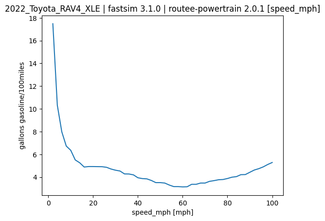
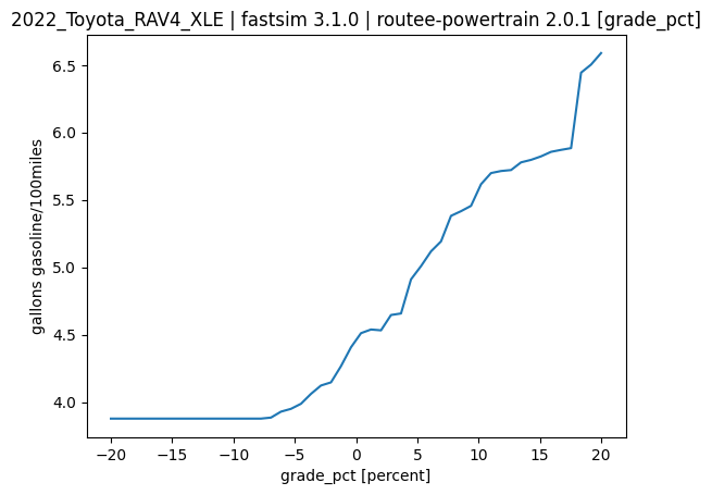
The first is the visualize_features function that sweeps a feature over a range and plots the results. In order to use this we first have to define what ranges the features should be considered.

feature_ranges = {
    "speed_mph": {"lower": 2, "upper": 100, "n_samples": 50},
    "grade_pct": {"lower": -20.0, "upper": 20.0, "n_samples": 50},
    # Every feature the model takes needs a range, distance included.
    "distance_mi": {"lower": 0.1, "upper": 1.0, "n_samples": 5},
}
results = pt.visualize_features(rav4, feature_ranges)

2026-09-11 21:54:46,571 [INFO] - Failed to extract font properties from /usr/share/fonts/truetype/noto/NotoColorEmoji.ttf: Can not load face (unknown file format; error code 0x2)

2026-09-11 21:54:46,602 [INFO] - generated new fontManager

<Figure size 640x480 with 0 Axes>

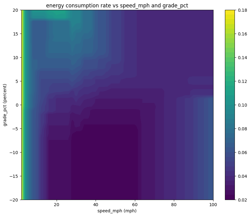
We can also look at two features simultaneously with the contour_plot function.

pt.contour_plot(
    rav4,
    x_feature="speed_mph",
    y_feature="grade_pct",
    feature_ranges=feature_ranges,
)