Deceleration Fuel Cut-Off Demo

This demo simulates a conventional vehicle over a drive cycle with and without Deceleration Fuel Cut-Off (DFCO), a feature that cuts off fuel flow while the vehicle is decelerating, and compares the resulting fuel economy.

import os
import sys
from pathlib import Path

import matplotlib.pyplot as plt
import pandas as pd
import seaborn as sns
from matplotlib.axes import Axes
from matplotlib.figure import Figure

sys.path.insert(0, str(next(p / "demo_scripts" for p in (Path.cwd(), *Path.cwd().parents) if (p / "demo_scripts").is_dir())))

import fastsim as fsim
from plot_utils import get_paired_cycler

sns.set_theme()

# if environment var `SHOW_PLOTS=false` is set, no plots are shown
SHOW_PLOTS = os.environ.get("SHOW_PLOTS", "true").lower() == "true"
# if environment var `SAVE_FIGS=true` is set, save plots
SAVE_FIGS = os.environ.get("SAVE_FIGS", "false").lower() == "true"

METERS_PER_MILE = 1609.34
MJ_PER_GGE = 125.0

Setup and Simulation¶

Run the same vehicle and drive cycle twice: once with DFCO disabled and once with DFCO enabled. The set_dfco_params method controls whether DFCO is enabled, the minimum speed at or above which it can activate, and the deceleration threshold required for it to activate.

# load 2026 Chrysler Pacifica Select with DFCO disabled
veh = fsim.Vehicle.from_resource("2026_Chrysler_Pacifica_Select.yaml")
veh.set_dfco_params(enabled=False, min_dfco_speed_m_per_s=0.0, max_accel_for_dfco_m_per_s2=0.0)
veh.set_save_interval(1)

# load cycle from file
cyc = fsim.Cycle.from_resource("udds.csv")

# instantiate `SimDrive` simulation object and run
sd = fsim.SimDrive(veh, cyc)
sd.walk()
df = sd.to_dataframe()

# load 2026 Chrysler Pacifica Select with DFCO enabled
veh_dfco = fsim.Vehicle.from_resource("2026_Chrysler_Pacifica_Select.yaml")
veh_dfco.set_dfco_params(
    enabled=True,
    # DFCO can activate at or above 11.176 m/s (25 mph)
    min_dfco_speed_m_per_s=11.176,
    # DFCO can activate when decelerating at 0.2 m/s^2 or more
    max_accel_for_dfco_m_per_s2=-0.2,
)
veh_dfco.set_save_interval(1)

sd_dfco = fsim.SimDrive(veh_dfco, cyc)
sd_dfco.walk()
df_dfco = sd_dfco.to_dataframe()

Fuel Economy Comparison¶

Compute fuel economy for both runs from cumulative fuel energy and cycle distance, then print the percent reduction in fuel use from DFCO.

cyc_dict = cyc.to_pydict()
distance_m = cyc_dict["dist_meters"][-1]
distance_mi = distance_m / METERS_PER_MILE

fuel_mj = df["veh.pt_type.Conv.fc.history.energy_fuel_joules"][-1] / 1e6
fuel_dfco_mj = df_dfco["veh.pt_type.Conv.fc.history.energy_fuel_joules"][-1] / 1e6

gge_gal = fuel_mj / MJ_PER_GGE
gge_dfco_gal = fuel_dfco_mj / MJ_PER_GGE
fuel_economy_mpg = distance_mi / gge_gal
fuel_economy_dfco_mpg = distance_mi / gge_dfco_gal

percent_reduction = (fuel_mj - fuel_dfco_mj) * 100.0 / fuel_mj

print(f"Conventional Vehicle Fuel Economy: {fuel_economy_mpg} mpg")
print(f"Conventional w/ DFCO             : {fuel_economy_dfco_mpg} mpg")
print(f"DFCO Reduction in Fuel Use (Conv): {percent_reduction} %")

Conventional Vehicle Fuel Economy: 23.89440188640568 mpg
Conventional w/ DFCO             : 24.52426480755952 mpg
DFCO Reduction in Fuel Use (Conv): 2.5683253956696874 %

Visualize Results¶

The following plot compares fuel converter behavior between the two runs.

def plot_fc_pwr(df: pd.DataFrame, df_dfco: pd.DataFrame, tag: str = "Conv") -> tuple[Figure, Axes]:
    """Plot fuel converter powers"""
    fig, ax = plt.subplots(3, 1, sharex=True, figsize=(10, 8))
    plt.suptitle("Fuel Converter Power")

    ax[0].set_prop_cycle(get_paired_cycler())
    ax[0].plot(
        df["cyc.time_seconds"],
        (
            df["veh.pt_type.Conv.fc.history.pwr_prop_watts"]
            + df["veh.pt_type.Conv.fc.history.pwr_aux_watts"]
        )
        / 1e3,
        label="f3 shaft",
    )
    ax[0].plot(
        df_dfco["cyc.time_seconds"],
        (
            df_dfco[f"veh.pt_type.{tag}.fc.history.pwr_prop_watts"]
            + df_dfco[f"veh.pt_type.{tag}.fc.history.pwr_aux_watts"]
        )
        / 1e3,
        label="f3 shaft (dfco)",
    )
    ax[0].set_ylabel("FC Power [kW]")
    ax[0].legend()

    ax[1].set_prop_cycle(get_paired_cycler())
    ax[1].plot(
        df["cyc.time_seconds"],
        df["veh.pt_type.Conv.fc.history.pwr_fuel_watts"] / 1e3,
        label="f3 fuel",
    )
    ax[1].plot(
        df_dfco["cyc.time_seconds"],
        df_dfco[f"veh.pt_type.{tag}.fc.history.pwr_fuel_watts"] / 1e3,
        label="f3 fuel (dfco)",
    )
    ax[1].set_ylabel("FC Power [kW]")
    ax[1].legend()

    ax[2].set_prop_cycle(get_paired_cycler())
    ax[2].plot(
        df["cyc.time_seconds"],
        df["veh.history.speed_ach_meters_per_second"],
        label="f3",
    )
    ax[2].plot(
        df_dfco["cyc.time_seconds"],
        df_dfco["veh.history.speed_ach_meters_per_second"],
        label="f3 (dfco)",
    )
    ax[2].legend()
    ax[2].set_xlabel("Time [s]")
    ax[2].set_ylabel("Ach Speed [m/s]")

    plt.tight_layout()
    if SAVE_FIGS:
        plt.savefig(Path("./plots/fc_pwr.svg"))
    if SHOW_PLOTS:
        plt.show()

    return fig, ax

Fuel converter shaft power, fuel power, and achieved speed for the baseline and DFCO runs. During decelerations above the minimum DFCO speed, the DFCO run’s fuel power drops to zero while the baseline continues to use idle fuel.

fig, ax = plot_fc_pwr(df, df_dfco)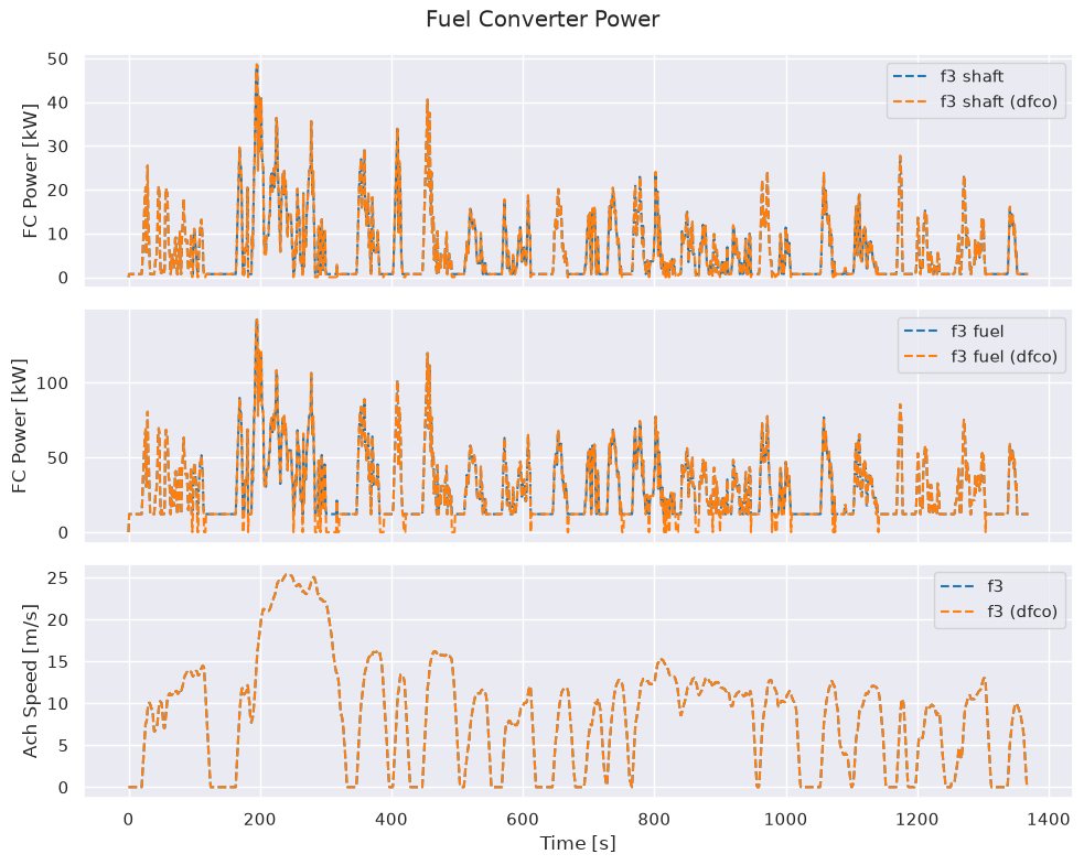

Source: fastsim/docs/demo_scripts/vehicle_controls/demo_dfco.py