Split-plot designs (hard-to-change variables)
This page shows how to mark variables that are slow or costly to change, generate a design that changes them as rarely as possible, run it in order, and keep them fixed when the optimizer suggests the next experiment.
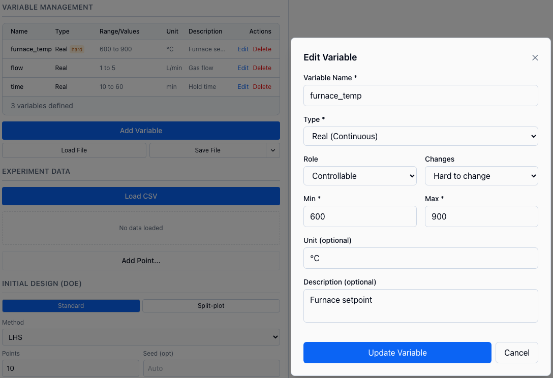
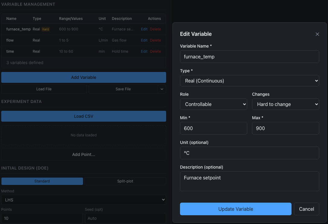
Marking a furnace temperature as hard to change.
When to use it
Some variables can be controlled but are changed rarely: a furnace that takes an hour to settle, a catalyst bed that is repacked once a day, a feed batch that lasts a week. If you reset every variable before every run, you do not need this page. If you cannot, a split-plot design groups the runs so that each hard setting is changed as few times as possible. The theory (whole plots, restricted randomization, why the analysis differs) is in Design of experiments.
1. Mark a variable as hard to change
- In the Variable Management panel, choose Add Variable, or Edit on an existing variable.
- Pick the Type and fill in the name and bounds as usual.
- Leave Role on Controllable. The Changes menu sits beside it; choose Hard to change or Very hard to change. Easy is the default.
- Choose Add Variable (or Update Variable). The variable list shows a hard or very hard badge.
Choosing Observed (measured) for Role declares a variable you measure rather than set, such as ambient temperature. Observed variables have no change level; see Observed variables.
One restricted level gives a split-plot design. Marking some variables hard and others very_hard gives a split-split-plot design with three levels.
2. Generate a split-plot design
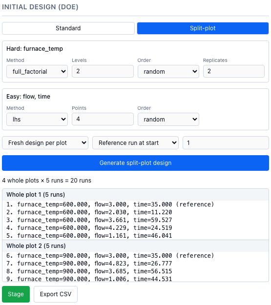
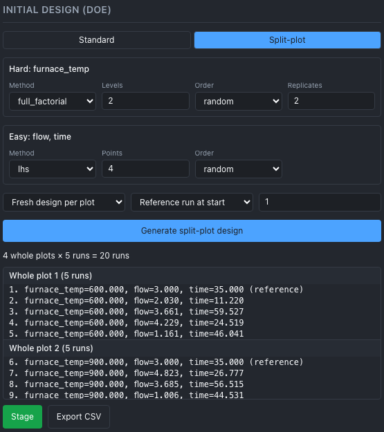
A split-plot design preview, grouped by whole plot.
- In Initial Design (DoE), choose Split-plot. The toggle between Standard and Split-plot appears only when a variable is hard or very hard.
- Each change level present has a card, such as Hard: furnace_temp. Set its Method, its Points or Levels, its Order, and for restricted levels its Replicates.
- Choose how the easy runs are drawn with Fresh design per plot or Same design in every plot, and a reference run with Reference run at start and end, Reference run at start or No reference run. A Seed (opt) makes the design reproducible. With a
very_hardvariable present, a further menu chooses between Fresh hard design per outer plot and Same hard design in every outer plot. The reference-run menu starts on Reference run at start and end, whereas the Python and RESTreferenceargument defaults toNone(no reference runs). - Choose Generate split-plot design. The preview is grouped as Whole plot 1 (5 runs) and so on, under a line such as "4 whole plots × 5 runs = 20 runs". Warnings appear in amber.
- Choose Stage to queue the runs for Add Point..., or Export CSV.
points, info = session.generate_split_plot_design(
    designs={
        "hard": {"method": "full_factorial", "n_levels": 2},
        "easy": {"method": "lhs", "n_points": 4},
    },
    replicates={"hard": 2},
    reference={"position": "start"},
    random_seed=7,
)
print(info["n_plots"], info["runs_per_plot"], info["n_runs"], info["warnings"])
print(points[0])
POST /api/v1/sessions/{session_id}/split-plot-design
Content-Type: application/json

{
  "designs": {
    "hard": {"method": "full_factorial", "n_levels": 2},
    "easy": {"method": "lhs", "n_points": 4}
  },
  "replicates": {"hard": 2},
  "reference": {"position": "start"},
  "random_seed": 7
}
The response holds points, n_points and info. Nothing is added to the session's data; the points are rows to run.
Every row has each controllable variable plus three or four bookkeeping columns.
| Column | Meaning |
|---|---|
WholePlot |
ID of the plot of the outermost restricted level. All rows with the same ID share one setting of those variables. IDs count from 1 across the whole design, and each replicate is a new plot. |
Subplot |
Present only with three levels: the ID of the hard plot inside a very_hard plot, again counted across the whole design. |
RunOrder |
1 to the number of runs, the order in which to run them. |
Reason |
Initial DoE (split-plot) for design rows, Reference (split-plot) for reference runs. |
How ALchemist does it
The generator nests the existing design methods, one per level, and info["warnings"] tells you when no whole-plot setting is replicated, so there is no pure-error estimate of the whole-plot variance. It does not analyze the data as a split-plot experiment: the Gaussian process ignores the plot columns. The method, the options and the limits are described under Split-plot designs.
3. Run the design in whole-plot order
Run the rows in RunOrder. You change the hard variables only when the WholePlot ID changes. In the web app, Add Point... steps through the staged rows in this order. When a row starts a new whole plot, a note reads "Whole plot 3 of 4: change the setup before this point", with the new value of each hard variable beneath it. Enter the response for each run, then choose Save N & close (N is the number of runs you entered). WholePlot, Subplot and RunOrder are stored with the data and are never model inputs.
In Python, pass the plot columns with each result:
def simulated_response(p):
    return -((p["furnace_temp"] - 780) / 100) ** 2 - ((p["flow"] - 3) / 2) ** 2 - ((p["time"] - 35) / 25) ** 2

for p in points:
    inputs = {name: p[name] for name in ("furnace_temp", "flow", "time")}
    session.add_experiment(
        inputs,
        output=simulated_response(p),
        reason=p["Reason"],
        plot={"WholePlot": p["WholePlot"], "RunOrder": p["RunOrder"]},
    )
print(len(session.experiment_manager.get_data()))
4. Hold a variable when suggesting
After training a BoTorch model, you can keep any controllable variable at a value for one suggestion, so the optimizer moves only the others. The usual use is to hold the hard variables at the furnace's current setting.
- In Acquisition Functions, find the Hold list. It appears when the model uses the BoTorch backend.
- Tick the box next to a variable and type its value (categorical variables use a menu). Or choose Hold current setup, which ticks every hard and very hard variable and fills in the values of the last recorded run.
- Choose Run Acquisition Strategy. A held variable shows a lock icon in the suggestion.
With anything held, the improvement baseline of EI, LogEI, PI, LogPI and qEI is the best posterior mean among the training inputs moved to the held values. Without a hold it is the best posterior mean at the training inputs themselves. A hold that leaves no point satisfying your constraints raises InfeasibleRegionError. Holds need the BoTorch backend and are rejected with qIPV and qNIPV.
The knowledge ratio
knowledge_ratio is the posterior standard deviation divided by the prior standard deviation of the model at the suggested point, noise excluded. It is near 0 where the data pin the function down and near 1 where the model has no information. Above 0.9, with something held or observed, warnings holds the text "the model has little information at these held values (knowledge ratio 0.94)". It means you asked for the best point at a setting the data say almost nothing about, so the suggestion is a guess. Run the design at that setting first.
| Result | Meaning |
|---|---|
knowledge_ratio of None |
The ratio was not computed: the sklearn backend, or a failure. |
Empty warnings |
The ratio is 0.9 or below, or nothing was held or observed. |
Observed variables
An observed variable is measured, not set: it is never optimized or put in a design, but the model uses it as an input, so each suggestion must say what it is now. Pass its current value as observed=. The older name context= still works; passing both raises an error.
import numpy as np

rng = np.random.default_rng(3)
obs_session = OptimizationSession()
obs_session.add_variable("furnace_temp", "real", bounds=(600.0, 900.0), changes="hard")
obs_session.add_variable("flow", "real", bounds=(1.0, 5.0))
obs_session.add_variable("ambient", "real", bounds=(15.0, 30.0), role="observed")
for temp in (600.0, 700.0, 800.0, 900.0):
    for _ in range(3):
        flow = float(rng.uniform(1, 5))
        ambient = float(rng.uniform(18, 26))
        y = -((temp - 780) / 100) ** 2 - ((flow - 3) / 2) ** 2 + 0.05 * ambient
        obs_session.add_experiment(
            {"furnace_temp": temp, "flow": flow, "ambient": ambient}, output=y
        )
obs_session.train_model(backend="botorch")
suggestion = obs_session.suggest_next(
    strategy="EI", goal="maximize", observed={"ambient": 22.5}
)
best = obs_session.find_optimum(goal="maximize", observed={"ambient": 22.5})
print(suggestion, best["x_opt"])
In the Hold list, observed variables appear under Measured now as required fields. The suggestion rows do not include observed variables; record their measured values with the result.
Options of generate_split_plot_design
session.generate_split_plot_design(designs, **kwargs) takes these arguments. designs has one entry per change level present (very_hard, hard, easy), each a design method plus its own arguments; any method of generate_initial_design works except optimal. Classical methods use n_center=0 unless you pass it.
| Argument | Default | Effect |
|---|---|---|
designs |
required | {level: {"method": ..., ...}}, exactly the levels present in the search space. |
replicates |
None (1 for each level) |
{"hard": 2} repeats that level's design; each repeat is a new plot. Restricted levels only. |
easy_mode |
"fresh" |
"fresh" draws a new easy design under each plot; "crossed" reuses one. "crossed" is refused if a constraint links the easy variables to an outer level. |
middle_mode |
"fresh" |
The same choice for the hard level when a very_hard level exists. |
reference |
None |
{"position": "ends"} (the default position) adds a reference run first and last in each innermost plot; "start" adds one first. "values" sets the easy variables; unnamed ones take the middle of their range, or the first level of a categorical. |
order |
None ("random" for each level) |
"random" shuffles plots, and for easy the runs inside a plot; "as_generated" keeps the generated order. |
random_seed |
None |
Makes the whole design reproducible. |
A design over 5,000 runs is refused. If an outer setting leaves no feasible inner design, the call raises InfeasibleRegionError naming the plot.